| On this page |
Blocks in Copernicus 
Blocks in the COP network act similar to compile blocks in the SOP network, as they encapsulate a bunch of nodes that you can treat as a single object. They typically consist of a ![]() Block Begin node and a
Block Begin node and a ![]() Block End, with other nodes in between. Turning on Simulate enables simulation mode, which ties the process to the frame bar, allowing for caching and checkpointing in memory for faster recooking and scrubbing.
Block End, with other nodes in between. Turning on Simulate enables simulation mode, which ties the process to the frame bar, allowing for caching and checkpointing in memory for faster recooking and scrubbing.
Another important feature is Live Simulation, which allows Houdini to continuously animate in almost real-time, providing real-time feedback for changes. This is similar to a video game world, where things play whether or not you are actively pressing anything. This mode is not tied to the playbar, but it’s still recooking all the time. So if you make a change in the network, you will see its results being played back live in the viewport.
Flow Blocks 
Flow blocks function like a 2D fluid solver, although no actual fluid is involved. It is basically a ![]() Flow Block Begin and a
Flow Block Begin and a ![]() Flow Block End with simulation mode turned on by default, and inputs/outputs for color, velocity, and temperature, are already set up. However, just like other blocks, you can turn off simulations, run fixed iterations, or enable live simulation.
Flow Block End with simulation mode turned on by default, and inputs/outputs for color, velocity, and temperature, are already set up. However, just like other blocks, you can turn off simulations, run fixed iterations, or enable live simulation.
Due to its 2D nature where everything has to rotate on a plane, it is not a real fluid simulation. While you could use this to make fire or smoke or liquid, it is generally intended to be an artistic tool to create interesting advection effects for motion graphics.
Using flow blocks 
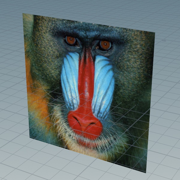
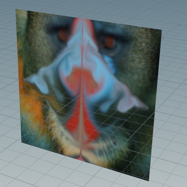
Once you use the tab menu to put down a Flow Block, you can put down a ![]() File. For this example, we will use
File. For this example, we will use Mandril.pic for the File Name. Then you can wire the c output of the File COP to the color input of the ![]() Flow Block Begin node. The following image is what you should see in the viewport.
Flow Block Begin node. The following image is what you should see in the viewport.
| To... | Do this |
|---|---|
|
Add some velocity |
|
|
Use temperature to drive simulation |
Tip You can use the Time Scale parameter on the
|
|
Blend in another image |
This will put the second File COP inside the block, which isn’t a problem for small files like this. However, if you were using a larger 2K or 4K texture, it would run significantly slower because it’s rerunning the file every frame. To solve this issue, you can instead use the |
|
Use collisions |
Note The flow solver uses a soft collision technique with a mask field. Increasing collision iterations will improve quality. The cache duration can be set on the Flow Block End node or managed with the |
|
Use divergence |
|
The other input/output of the Flow Block is feedback. Color, velocity, and temperature are all fed back by default. This input lets you have extra fields, if you need more than just these three.
Note
feedback and passthrough don’t have to be a single layer. These two inputs can accept cables as well.
Content library example 
|
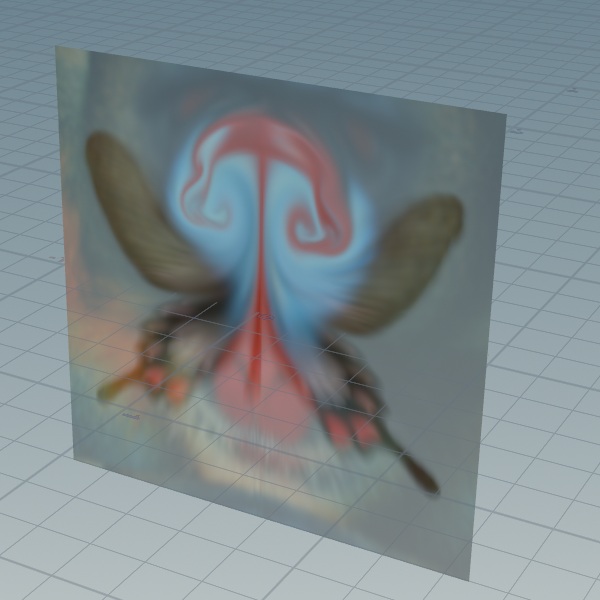
The Houdini 21 splash screen project demonstrates the Flow Solver working in synergy with both SOP and DOP contexts. It shows how you can generate organic, intricate velocity fields in just a few minutes and then apply that data across different areas of Houdini. Download the file here. |
|---|