| On this page |
|
Step 0 - Getting started 
This page assumes you've read and completed the getting started page for this tutorial, which explains how to load the example asset you will follow along with. If you haven’t loaded the asset yet, go to that page first.
Step 1 - Build Materials 
Tip
You might find it useful to have a pinned parameter pane displaying the buttons on the example always visible.
-
In the network editor, right click the asset (
rbd_mf_tutorial1) and choose Parameters and Channels ▸ Parameters to open the node’s parameters in a floating window.
On Linux, depending on your window manager, you might also want to use the window manager UI to tell the window to stay on top of other windows.
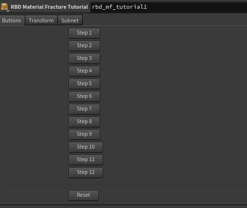
To start, click the Reset button on the example asset (the last button).
This will delete all the nodes inside the wall object except the wall1 subnet SOP. (You will spend the reset of the tutorial recreating the simulation step-by-step.)
Click the Step 1 button.
There may be a delay while Houdini creates three ![]() RBD Material Fracture SOPs and configures them for you.
RBD Material Fracture SOPs and configures them for you.
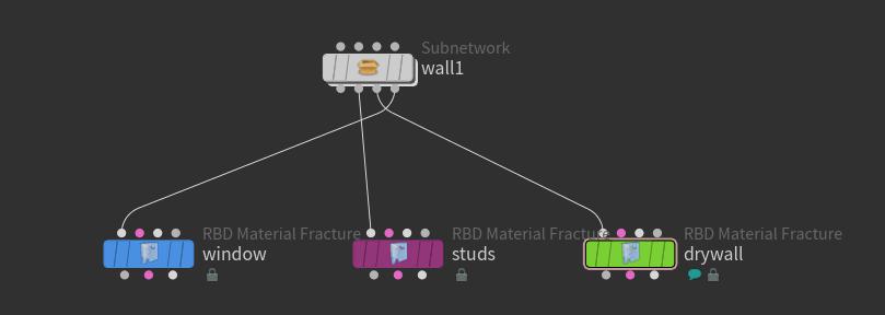
Let’s take a look at the RBD Material Fracture SOPs and see how they are set up and make some changes. We will not examine every single parameter, just the ones that are of interest and/or not set to their defaults.
window node
The first RBD Material Fracture SOP is called “window”. It is a good idea to rename your SOPs to something descriptive. We have also color-coded the node and any other nodes that relate to it so that they are easier to associate.
Parameter |
Value |
Notes |
|---|---|---|
Material type |
Glass |
We want to create the material for the window, so we used the Glass menu option. |
Fracture namespace |
|
It is ideal to have geometry that already has unique primitive name attributes. If you already have these attributes, you do not need to (nor do you probably want to) toggle on namespaces in this SOP. In our case, our geo does not have any To see what is happening, right-click the node, and choose, Spreadsheet. Look at the Primitive attributes only and note they are all prefixed with "window.” Now turn off the Fracture Namespace checkbox and you will see they are prefixed with “piece”.
|
Fracture per piece |
|
In this case there’s only one “piece”, (one pane of glass), so it doesn’t matter if this is on or off. Note that if your geometry already has a “name” attribute, you can tell this SOP to examine each chunk of geo with the same name attribute one at a time. If there is no name attribute, it will simply use the connectivity to determine the “chunks” to work on. See the notes on the “studs” for more on this. |
Constraints Tab 
Parameter |
Value |
Notes |
|---|---|---|
Apply Constraint Properties |
|
We are going to apply the properties later on down the chain, so it does not matter if we set these since we are going to overwrite them later. |
-
You will see that each RBD Material Fracture SOP has four inputs and three outputs. If you mouse over them, you will see what they are:
Geometry
The high-res geometry.
Constraints
Any constraints you have created.
Proxy Geo
The low-res geometry.
Extra Vornoi Points
Extra points to add to the Vornoi points for concrete, impact points for glass, or cutter geometry for a custom material type.
Houdini actually simulates the low-res geometry. After the simulation, the
 RBD Bullet Solver SOP transforms the high-res geometry to match the simulated low-res geometry. It does this by matching the name attributes on the two geometry streams.
 -
If you right-click and select the Geometry Spreadsheet on one of these SOPs, you can examine any of these streams of geo via the dropdown menu.
-
You can also examine these streams with an
 RBD Exploded View SOP.
 -
Another way to examine and/or isolate a stream is by piping it out to a
 Null SOP.
 -
You can also use the “Output for view” flags, (hotkeys 1, 2 and 3 when in RBD State, or
 on the RBD Bullet Solver SOP → Flags → Output for view.
studs node
Parameter |
Value |
Notes |
|---|---|---|
Material type |
Wood |
The “studs” (or “framing”) of this structure will be wood. |
Fracture namespace |
|
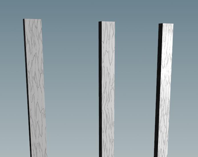
Look closely at the wood pattern. Notice that the wood grain is running vertically, as you would expect it to. Houdini loops through each connected piece of geometry, (or uses the Piece Attribute if there is one) and orients the fractures along the bounding box. In this case, since these studs are long and thin, it does the right thing.
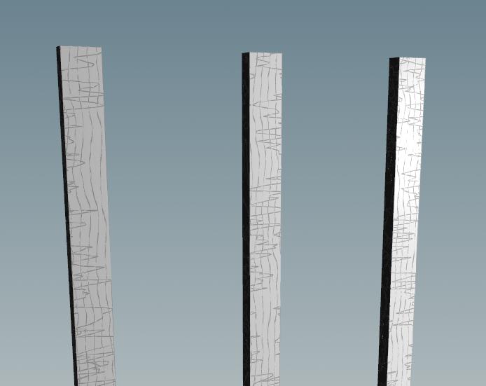
Turn off Fracture per Piece. Be prepared for the node to take some time to cook after you do this. If you do not have a fast machine, you may want to skip this step.
Note that the wood grain is now horizontal, which is not right. So what happened here? Because we don’t have Fracture per Piece turned on, Houdini looks at the seven studs and thinks that is one big piece of wood with holes in it, oriented horizontally, wider than it is high.
Now turn Fracture per Piece back on.
Note that, first, the node cooks much more quickly. Second, the grain is oriented properly. This is because Houdini goes through each connected chunk of geometry and examines it individually. You can prove this buy turning on the Single Pass parameter. You will see that it only does one stud at a time.
Cluster tab 
Parameter |
Value |
Notes |
|---|---|---|
Enable cluster |
|
To see what this does, append a
Now turn on Enable Cluster. When clustered, the RBD Material Fracture node gives some adjoining pieces the same name attribute so they will be treated as one “piece” when they are simulated. In this case, we don’t want this, but in some cases it can make for more interesting shapes.
Turn Enable Cluster back off. |
Tip
Another way to cluster is by using the ![]() Cluster SOP. This node can cluster either geometry or constraints.
Cluster SOP. This node can cluster either geometry or constraints.
drywall node
Parameter |
Value |
Notes |
|---|---|---|
Material type |
|
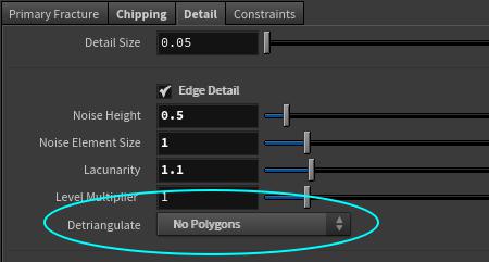
We want to create drywall material, and the closest material to this in the RBD Material Fracture SOP is concrete. Later on we will configure this to have the physical properties of drywall. We have turned on the Chipping and Detail options to give this a more interesting shape and detail. Feel free to play with these options the next time you do this tutorial to see how the shape of the cuts change. |
Fracture namespace |
|
Note that this object has a boolean in it. If the object, after it goes through the RBD Material Fracture SOP, has artifacts in it (bad geometry), go to the Detail tab and change the Detriangulate parameter to No Polygons or Only Unchanged Polygons. The Detriangulate options turn the geometry back into n-gons, but this sometimes does not work with booleaned or very complex geo.
The above option usually fixes bad geometry. However, if it doesn’t work, try the following one at a time in various orders:
-
Apply Polycap SOPs to cap any unclosed surfaces.
-
Reverse the geo with a
 Reverse SOP.
 -
Try
 Fuse SOP and/or
  Polydoctor SOP.
 -
Apply a
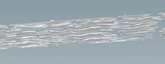
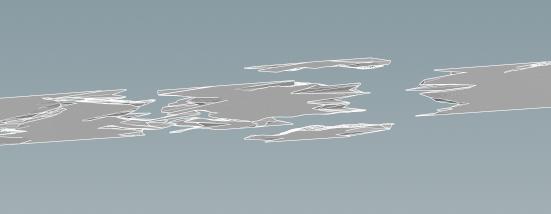
 Divide SOP with Convex Polygons turned off, and Bricker Polygons turned on to dice up the geo (see image below). You may need to apply another Divide SOP (at the default settings) after this to triangulate the geo.
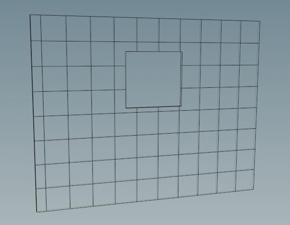
Above we see the geometry brickered by the ![]() Divide SOP.
Divide SOP.
Step 2 - Merge the Materials 
Click the Step 2 button.
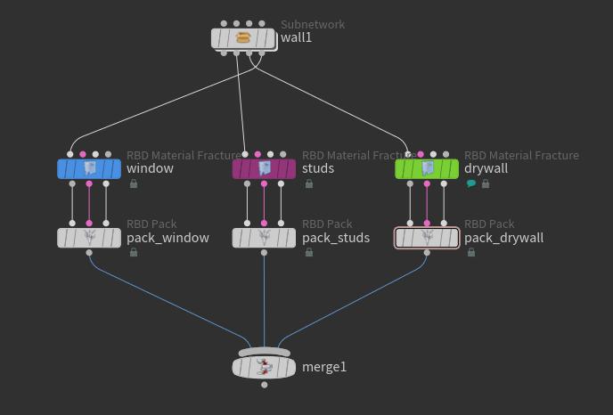
We now have three ![]() RBD Pack SOPs and a
RBD Pack SOPs and a ![]() Merge SOP. The RBD Pack nodes simply take care of packing up the three streams of geometry so you can can merge them. We will unpack them shortly.
Merge SOP. The RBD Pack nodes simply take care of packing up the three streams of geometry so you can can merge them. We will unpack them shortly.
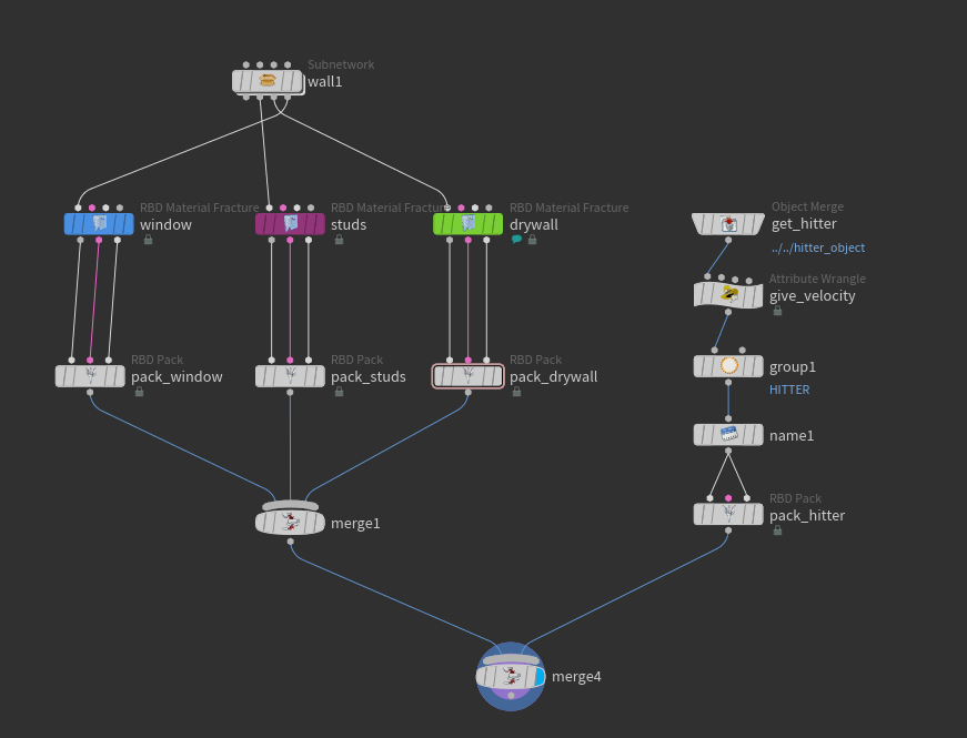
Step 3 - Add a Hitter 
We are going to add a simple object as a “hitter”. Of course, there are a limitless number of ways to interact with an RBD simulation, either by having object(s) with velocity hit other objects, keyframing objects, dropping objects, using forces, etc. In this tutorial, we will give a random object some velocity so that it slams into the wall.
Click the Step 3 button.
Let’s examine this node network.
Object merge node 
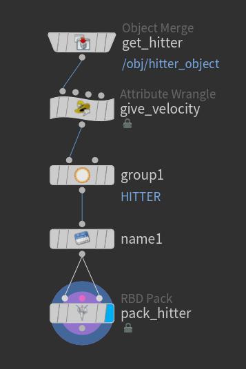
The first SOP in the chain is a ![]() Object Merge SOP.
Object Merge SOP.
Parameter |
Value |
Notes |
|---|---|---|
Object 1 |
|
We are simply getting a sphere from the object level to use as a hitter. |
Transform |
Into This Object |
Switch this parameter to None to see that it will ignore the object-level transforms. Change it back to Into This Object, as we have transformed this sphere at the object level and need these transforms. |
Attribute wrangle node 
The second SOP in the chain is an ![]() Attribute Wrangle SOP. We are going to add velocity to the object by using the following VEX code:
Attribute Wrangle SOP. We are going to add velocity to the object by using the following VEX code:
v@v=set(0,0,-35);
Here we are adding some velocity in Z so that the sphere will hit the wall and destroy it.
Tip
Middle-click the node to see that you now have a v attribute. You can also right-click to view the Geometry Spreadsheet and examine the point velocity’s actual values. As a Houdini artist, you will use these techniques often to examine and/or confirm attribute values.
Tip
Instead of using a Point Wrangle SOP, you could use a ![]() Point Velocity SOP.
Point Velocity SOP.
Group node 
The third SOP in the chain is a Group SOP.
Here we are naming this object HITTER. Putting your objects in easily-identifiable groups will make working with them later much easier.
Name node 
The fourth SOP in the chain is a ![]() Name SOP.
Name SOP.
Parameter |
Value |
Notes |
|---|---|---|
Name |
|
Bullet deals with objects via their name attribute. Each RBD object needs to have a unique name. If the name attributes are duplicated, you will get unpredictable and incorrect results. This is why we need to give this object a primitive “name” attribute. |
RBD Pack node 
The fifth SOP in the chain is an ![]() RBD Pack SOP.
RBD Pack SOP.
We have wired the ![]() Name SOP into the first and last inputs of the
Name SOP into the first and last inputs of the ![]() RBD Pack SOP. Hover your mouse over these inputs to see what the SOP is expecting. In this case, it’s expecting (from left to right):
RBD Pack SOP. Hover your mouse over these inputs to see what the SOP is expecting. In this case, it’s expecting (from left to right):
Geometry
The high-res geometry.
Constraints
Any constraints you have created (in this case none).
Proxy Geo
The low-res geometry.
In this case, the high-res and low-res geo are the same, so we connect the same geo into both inputs.
Your network should now look like this:
Step 4 - Unpack 
Click the Step 4 button.
This adds a ![]() RBD Unpack SOP, so we can continue to tweak our network.
RBD Unpack SOP, so we can continue to tweak our network.
Step 4a - Save to Disk 
This section is optional, but recommended. It is a good idea to save your geometry to disk after creating your materials using the RBD Material Fracture nodes. Fracturing materials can be a lengthy process, and you don’t want to have to wait for these nodes to cook every time you open a file.
In this case, you can add a ![]() File Cache SOP,
File Cache SOP, ![]() File SOP or a
File SOP or a ![]() RBD I/O SOP to your chain to save your geo to disc. By caching the geo to disc, the nodes above will not have to cook unless you re-create any of the materials above.
RBD I/O SOP to your chain to save your geo to disc. By caching the geo to disc, the nodes above will not have to cook unless you re-create any of the materials above.
There are two places you can do this:
-
After each
 RBD Material Fracture SOP.
This will give you more flexibility later if you want to change only one material. This way you can save that one material without having to cook the other two unchanged nodes.
-
After you merge all of the RBD Material Fracture nodes (as seen below).
This is slightly easier to set up, but at the expense of flexibility.
In the image below, we did not cache the hitter object to disc. This object is very light-weight, and we will probably want to continually tweak its velocity to get the best results.
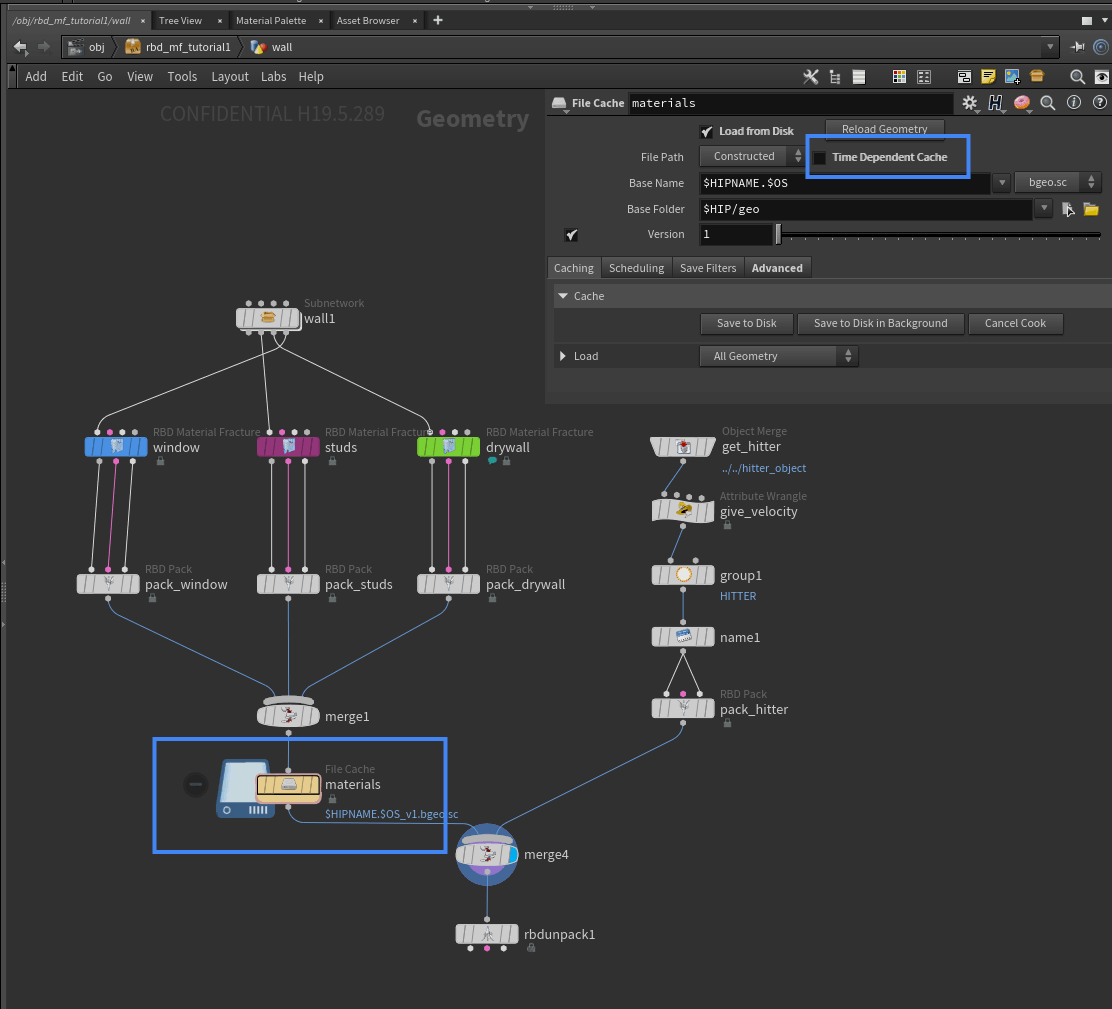
Note
You only have to save ONE frame to disc, so toggle OFF “Time Dependent Cache” if you are using the File Cache node. The pre-fractured geometry is not animated so there is no need to save out more than one frame.
Step 5 - Simulate 
Go to Frame 1. We do this before we are about to simulate, so we don’t have to wait for the whole timeline to cook.
Click the Step 5 button.
This adds an ![]() RBD Bullet Solver SOP with some static geometry connected into the fourth input to use as a static collider, (the vertical beams).
RBD Bullet Solver SOP with some static geometry connected into the fourth input to use as a static collider, (the vertical beams).
Note
The node is way down at the bottom of the network pane. This is to leave room for the other SOPs we will be adding.
The ![]() RBD Bullet Solver is a wrapper around a DOP network to simplify the running of Bullet simulations. Inside this network is a series of nodes that simplifies the setup of an RBD Solve. This takes a lot of the grunt work out of building the simulation, managing constraints, working with high and low-res geometry, and also gives you access to great visualization and debugging tools. It also allows the easy integration of guided simulations.
RBD Bullet Solver is a wrapper around a DOP network to simplify the running of Bullet simulations. Inside this network is a series of nodes that simplifies the setup of an RBD Solve. This takes a lot of the grunt work out of building the simulation, managing constraints, working with high and low-res geometry, and also gives you access to great visualization and debugging tools. It also allows the easy integration of guided simulations.
Make sure the display flag is turned on the newly created ![]() RBD Bullet Solver SOP.
RBD Bullet Solver SOP.
Click ![]() Play Forward in the playbar.
Play Forward in the playbar.
The wall simply drops through the floor.
Navigate to the Ground subtab turn on Add Ground Plane. This is located on the Solver tab of the newly created ![]() RBD Bullet Solver.
RBD Bullet Solver.
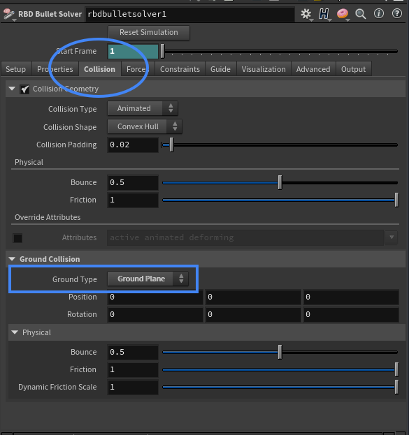
Play the simulation again.
It is slightly better, but every material is very weak and nothing is attached to anything else.
Step 6 - Constraints between materials 1 
Note
When talking about material constraints, we often refer to constraints within a material (holding together pre-fractured pieces), and constraints between materials (for example, holding a window in a frame). Constraints within a material are called intra-material constraints. Constraints between different materials are called inter-material constraints (intra means within, inter means between in Latin). The similarity between the two words may be confusing, but these terms are often used in production so we will use them here.
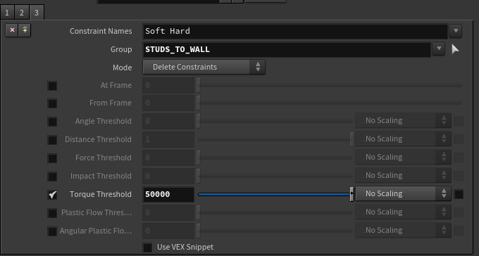
Studs to Wall 
The RBD Material Fracture SOPs have created the constraints within materials (intra-material constraints). These are the constraints that define the strength of the bonds between the pre-fractured geometry. For example, how strong and resistant to fracture the drywall is.
Each of these individual SOPs have no idea what objects exist outside of them, and how the materials that have been created should be attached to each other. This is why we need to create inter-material constraints. For example, we want the drywall constrained to the studs, (in the real world, the drywall would be screwed or nailed to the studs), and we want the window glass to be constrained to the drywall, (in the real world, it would be sandwiched into a frame which would be glued/screwed into the wall opening). Getting these constraints right is vital to a good-looking simulation.
We are going to use various SOPs to create and configure these constraints.
Click the Step 6 button.
This creates an ![]() RBD Constraints From Rules SOP and an
RBD Constraints From Rules SOP and an ![]() RBD Constraint Properties SOP.
RBD Constraint Properties SOP.
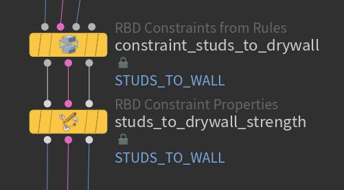
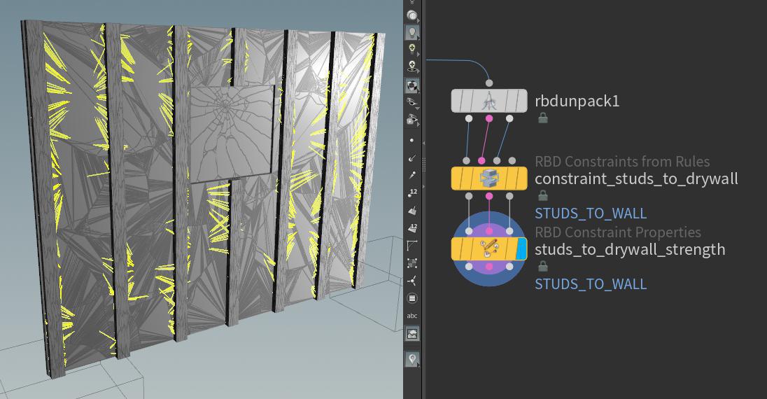
In the first SOP (![]() RBD Constraints From Rules),
RBD Constraints From Rules), constraint_studs_to_drywall, we create a group called STUDS_TO_WALL by using the Group to Group option and the existing groups, drywall and studs.
Parameter |
Value |
Notes |
|---|---|---|
Group Name |
|
|
Groups |
|
|
Group 1 |
|
|
Group 2 |
|
In the second SOP, (![]() RBD Constraint Properties), we simply color the constraints yellow and ensure that the existing constraints are Glue constraints and have a strength of
RBD Constraint Properties), we simply color the constraints yellow and ensure that the existing constraints are Glue constraints and have a strength of 10,000. This ensures we can control these constraints here, after the ![]() RBD Constraint From Rules SOP has created the constraints for us.
RBD Constraint From Rules SOP has created the constraints for us.
If you display this SOP and look in the viewport, you will see the yellow constraints.
Step 7 - Constraints between materials 2 
Window to Drywall 
We are now going to constrain the window to the drywall. Of course, in reality the window would be glued to a frame, and the frame nailed to the studs. For simplicity’s sake, we will go with this scheme.
Click the Step 7 button.
As in the previous step, we created ![]() RBD Constraints From Rules SOP and an
RBD Constraints From Rules SOP and an ![]() RBD Constraint Properties SOP to create new constraints between materials (inter-material constraints) and set their properties.
RBD Constraint Properties SOP to create new constraints between materials (inter-material constraints) and set their properties.
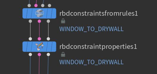
In the ![]() RBD Constraints From Rules SOP we created new constraints and a unique group, this time,
RBD Constraints From Rules SOP we created new constraints and a unique group, this time, WINDOW_TO_DRYWALL. This time we were able to identify the two groups by using the following syntax:
@name=window* and @name=drywall*
This means, if the name attribute begins with “window”, include it in this section and if the name attribute begins with “drywall”, include it in this section.
In the second SOP, (![]() RBD Constraint Properties), we again just set default Glue constraints.
RBD Constraint Properties), we again just set default Glue constraints.
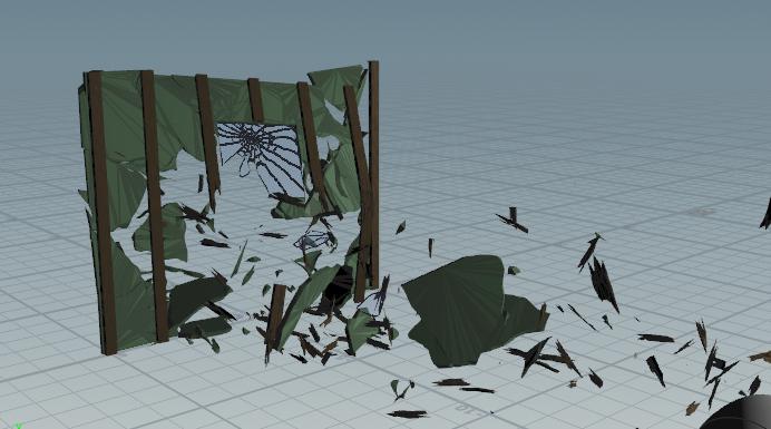
Review Simulation 
Play the simulation.
It definitely looks better, but it could still be improved. Here’s a few ideas of what might make it better:
-
The studs should be “nailed” to the floor. Right now they are frictionless and don’t interact with the ground at all.
-
The glass does not break easily enough.
-
The hitter needs more power.
-
The studs just break like glass. It would be better if they bent before they break.
-
Same for the drywall. It would be nice to see it bend before it breaks.
-
Some of the studs would look better if they snapped in half.
Step 8 - Tweak constraints between materials 
Our studs already have constraints within the material (intra-material constraints) that define their strength (resistance to breakage). However, we will want to tweak these values as we play with the simulation. We are able to do this with another ![]() RBD Constraint Properties SOP.
RBD Constraint Properties SOP.
Click the Step 8 button.
This adds another ![]() RBD Constraint Properties SOP and two
RBD Constraint Properties SOP and two ![]() RBD Configure SOPs.
RBD Configure SOPs.
The RBD Configure SOP lets you set up properties individually for different sets of RBD objects. The Physical Attributes controls are very useful, as there are many predefined density, friction, and bounce settings for different material types derived from engineering textbooks, which will give you a head start on getting results that are physically realistic. See ![]() the docs on this node for more details.
the docs on this node for more details.
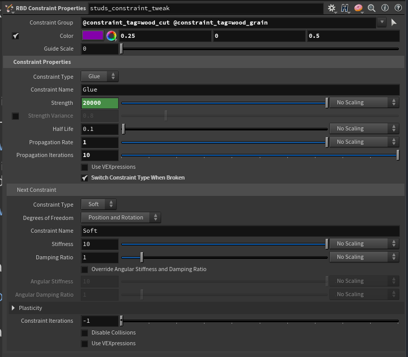
studs_constraint_tweak node
Parameter |
Value |
Notes |
|---|---|---|
Constraint Group |
|
The
|
We have now tweaked the constraints so that when the Glue constraints break, they become Soft (springy) constraints. This will give the illusion that the wood bends before it breaks.
make_bottom_of_studs_non_active SOP
We have also added an ![]() RBD Configure SOP to “nail” two of the studs to the floor. We do this by making the bottoms of the studs inactive. These inactive pieces will still act as collision object in the sim, they just won’t be simulated themselves.
RBD Configure SOP to “nail” two of the studs to the floor. We do this by making the bottoms of the studs inactive. These inactive pieces will still act as collision object in the sim, they just won’t be simulated themselves.
Parameter |
Value |
|---|---|
Group |
|
Active |
|
Use Bounds |
|
Physical Attributes |
Wood, Pine, Dry and Clean Surfaces |
Density, Bounce, Friction |
|
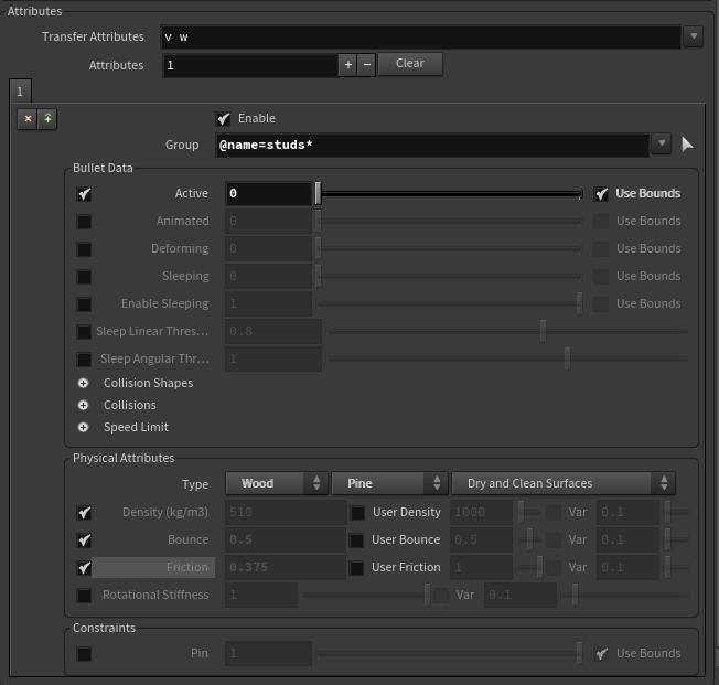
Note
When using the physical attribute presets, you must enable the various Density, Bounce and/or Friction parameters you are interested in for the preset to have an effect.
configure hitter SOP
Let’s configure the hitter object so it has the properties of clean, dry metal.
Parameter |
Value |
|---|---|
Group |
|
Type |
Metal, Default, Clean and Dry Surfaces |
Density, Bounce, Friction |
|
Check Simulation 
Go to frame 1, and on the ![]() RBD Bullet Solver, press Reset Simulation, and then play the sim. It’s looking better, but now the studs look like wet spaghetti. This is because the soft constraints never break.
RBD Bullet Solver, press Reset Simulation, and then play the sim. It’s looking better, but now the studs look like wet spaghetti. This is because the soft constraints never break.
Tweak Breaking Thresholds 
We need to tweak the RBD Bullet Solver’s breaking thresholds for the wood pieces. Go to the Breaking Thresholds tab and set the following:
Parameter |
Value |
Notes |
|---|---|---|
Group |
|
You can choose these groups from the drop-down menu. Tip Use the constraint browser to identify these constraints as being the ones that belong to the wood parts we are attempting to modify. |
Impact Threshold |
|
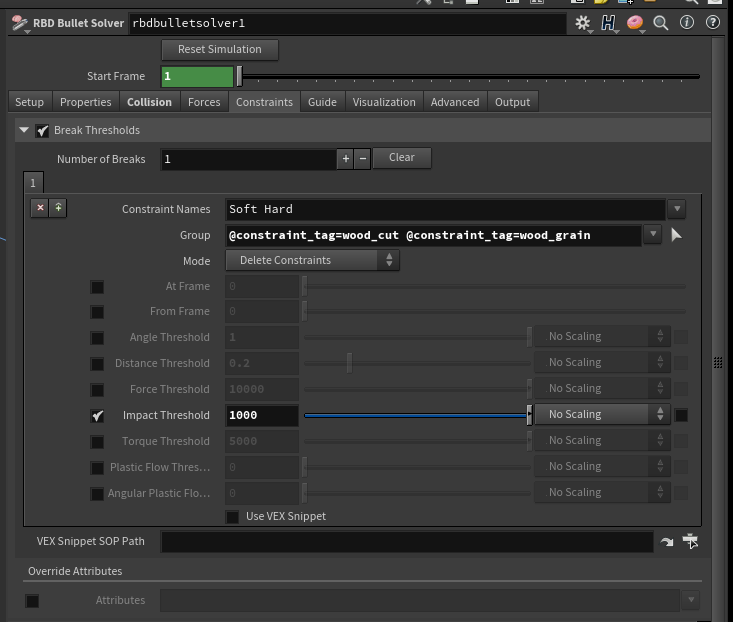
Play the sim again. Now the wood is breaking too easily. Use the Visualize tab to determine the right value for the breaking threshold.
Using the Visualize Tab 
We need to see the impact values that the constraints have. When we get an idea of what these values are, we can then decide where we should set the breaking thresholds.
Go to the Visualize tab of the ![]() RBD Bullet Solver.
RBD Bullet Solver.
Parameter |
Value |
|---|---|
False Color Mode |
|
Attributes |
|
Float Precision |
|
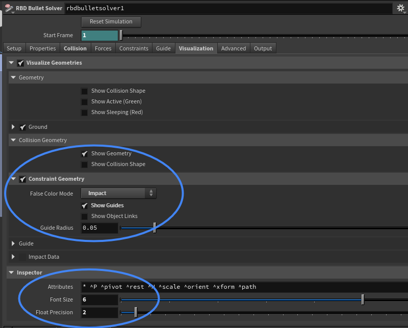
Go to about frame 40 of your sim. In the viewport, with the RBD Bullet Solver selected, press Enter to enter the ![]() RBD Bullet Solver visualization mode. You should now see a false-color graph at the top of the viewport that shows you the ranges of impacts in the scene.
RBD Bullet Solver visualization mode. You should now see a false-color graph at the top of the viewport that shows you the ranges of impacts in the scene.
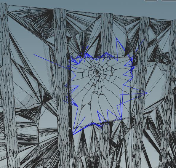
In the viewport, press the 5 key. This toggles on the inspector. Hover your mouse over the sim. You should see the “name” attribute of the piece under the mouse.
Now, in the viewport, press the 2 key. This puts you in Constraint Viewing mode. The modes are:
1 |
Geometry (high-res) View |
2 |
Constraint View |
3 |
Proxy Geometry |
You can now see the impact values of the constraints holding the pieces of wood together. Depending on your scene, these might be in the range of 10,000 to 50,000.
In the video below, we hit ⎋ Esc then Enter to go into the visualization mode. Then we hit 5 to enter visualization mode, then 1 to go to hi-rez geo, 2 for constraints, 3 for proxy geo, then back to 2 for constraints and then hover over the geo to see info.
Start by setting the Impact Threshold to 10000. Play the scene a few times and see how it looks. This value is probably too low. Keep playing with it until you get something fairly pleasing. We are looking for a situation where some wood breaks and some bends but does not break. Don’t spend too much time on this, as we have further tweaking of other constraints to do, and we will have to change these values later on.
For this tutorial, set the Impact Threshold at about 45000.
Tip
By default, you are going to see almost all the attributes in the viewport. If you are only interested in looking at impact for example, just put impact in the Attributes field of the inspector instead of the default * ^P ^pivot ^rest ^N ^scale ^orient ^xform ^path.
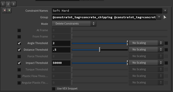
Step 9 - Configure the Drywall and Glass 
We now have to configure the drywall and glass to have the physical properties of these materials.
Click the Step 9 button.
This adds the following nodes:
-
 RBD Constraint Properties SOP:
 drywall_constraints_tweak -
RBD Constraint Properties SOP:
glass_constraints_tweak -
 RBD Configure SOP:
 glass_tweak
Examine these SOPs to see how they have been set to give the material and the constraints realistic values.
Tips for Refining Your Simulation 
| To... | Do this |
|---|---|
|
Control how easily something breaks |
Tweak Glue Strength |
|
Make things bend before they break |
Use both Glue and Soft constraints. |
|
Control springiness |
Tweak Stiffness and Damping Ratio. |
|
Make sure springy things actually break |
Identify the constraints (name and type), and constraint values, and tweak the breaking thresholds, (as described above). |
|
Determine how sticky things are |
Use the Physical Attributes section on the |
|
Spread the impact far enough along the structure |
Tweak the Propagation Iterations and Half-life parameters. See the |
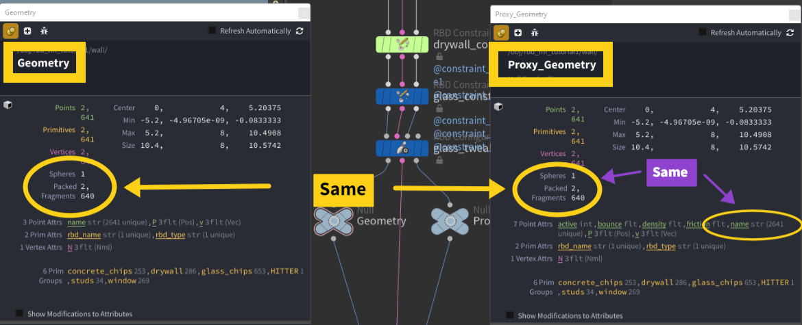
It is often a good idea to pipe the outputs of three-output SOPs into nulls and then examine them individually.
-
Look at the geometry via the Geometry spreadsheet.
-
Middle-click the node to see what attributes exist.
-
Blast away groups to ensure they contain what you think they contain.
-
Blast away geometry via an expression to see if the attributes have the value you think they should have. For example,
@strength>10000.
Parameter |
Value |
Notes |
|---|---|---|
Propagation Iterations |
|
|
Propagation Iterations |
|
|
Continue to Refine the Simulation 
We will continue to play the simulation and refine the values of the various material properties, constraint properties, and breaking thresholds.
You may notice that the wood is still springy looking and some of the constraints are not breaking. Let’s go back and examine the constraints.
Play the sim to a point where you see some strange wood behavior.
Using the previously described technique, examine the constraints for the wood. In this case, we want to change the attributes we are examining. In the ![]() RBD Bullet Solver’s Visualize tab, right-click the Attributes parm and choose, Revert to defaults. This will show all attributes except for the ones with the “caret” ^ sign in front of them.
RBD Bullet Solver’s Visualize tab, right-click the Attributes parm and choose, Revert to defaults. This will show all attributes except for the ones with the “caret” ^ sign in front of them.
Go back to the Breaking Threshold tab. You will notice that there are a lot of different value attributes we can use to break the constraints. The ones we might be interested in are below, with some suggested values arrived at after much experimentation.
Parameter |
Value |
Notes |
|---|---|---|
Angle |
|
(Breaks anything that bends beyond |
Distance |
|
(Breaks anything that stretches beyond |
Force |
|
|
Impact |
|
(Breaks anything with an impact value of |
Torque |
|
(Breaks anything with a torque (angular velocity) value of |
Tip
Hover your mouse over the labels to get an explanation of what they are measuring.
Step 10 - Fine Tune Constraints 
After looking at your sim, you or your supervisor may say, “This looks great, but I want this thing to break here, and this one to break here.” There is an easy way to do this.
Click the Step 10 button.
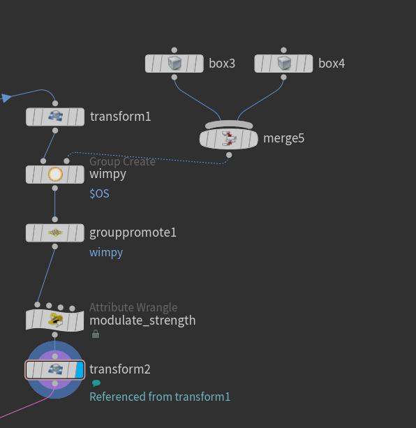
This adds the following node network:
Moves the studs out of the way so they are easier to select and isolate.
Allows grouping of the constraints.
Note
You can also group the nodes by simply selecting the geometry interactively. However, the method used here is a more robust way of doing it, as the selection will not change if you make changes to your constraints at another time.
Promotes the above point group to a primitive group. Bounding box grouping only works on points, but we want to modify primitive attributes.
Sets the group’s Glue Strength to a very low value so these constraints will break easily.
We are simply setting the strength value of the group “wimpy” (created above) directly: @strength=100;.
To move the constraints back to where they used to be.
This SOP was created by choosing the transform1 SOP above, right-clicking and choosing Actions ▸ Create Reference Copy. On the Invert Transformation checkbox, right-click and select Delete Channels, so it’s no longer linked to the Transform SOP above, and turn on Invert Transformation.
More Tweaking 
Here are a few suggestions. Tweak these one at a time to see what they do to your simulation. It is also a good idea to go extreme on these setting sometimes to see what effect they might have.
-
In the
rbdconstraintproperties1SOP, set the Glue Strength to500. -
In the
rbdbulletsolver1SOP: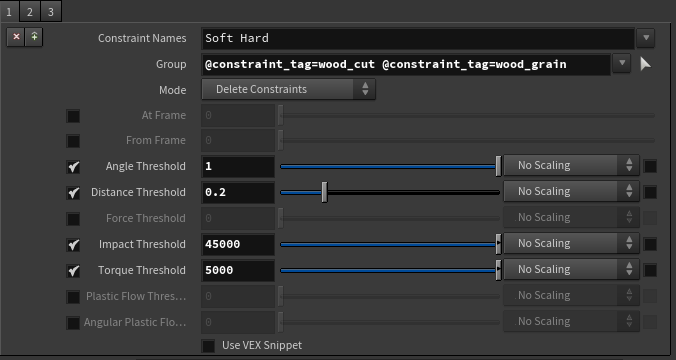
Step 11 - Add Materials 
Click the Step 11 button.
This adds materials to your network. We won’t examine this in detail, but feel free to explore this section.
Step 12 - Tweak Glass 
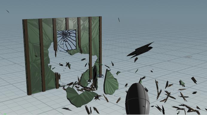
If you go to frame one and you render your scene now, (render through cam2 for a close-up of the glass), you will notice that the window glass appears broken before it visually shatters. Of course, all of the geometry is pre-broken, but we don’t want our viewers to know this.
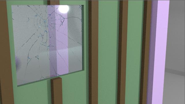
The reason the glass appears broken is because it is both transparent and refractive. This means that we see the inside edges of the broken glass, which refract and break-up light when they are rendered. In order for the glass to appear non-shattered, we need to hide these inside edges until we want them to be seen.
Click the Step 12 button.
This adds nodes in two places. The first is at the top left of the network.
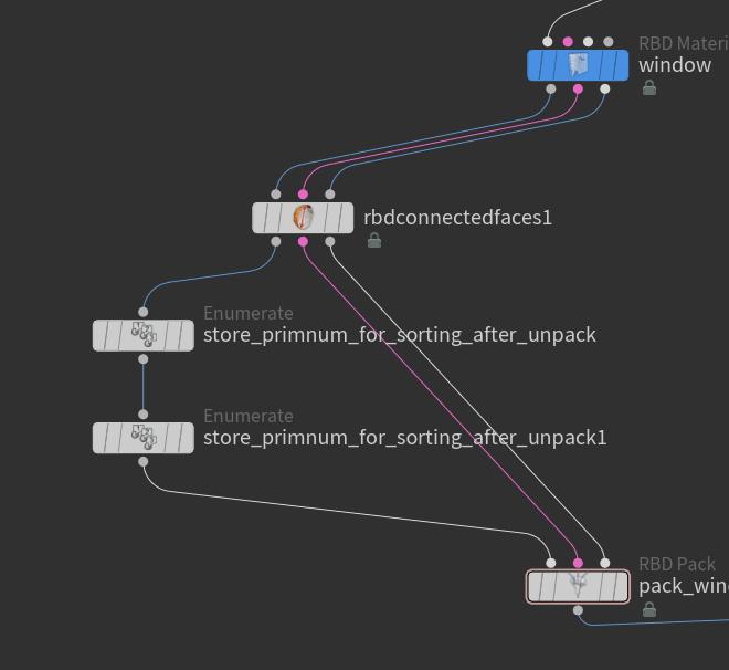
The ![]() RBD Connected Faces SOP stores information about connected inside faces to help determine if these faces have become separated by the process described next. The two
RBD Connected Faces SOP stores information about connected inside faces to help determine if these faces have become separated by the process described next. The two ![]() Enumerate SOPs set an attribute on each point or primitive in the selected Group sequentially, (see the node help for more info). We are going to use this information later to sort our geometry so that the nodes below know which geometry to act on.
Enumerate SOPs set an attribute on each point or primitive in the selected Group sequentially, (see the node help for more info). We are going to use this information later to sort our geometry so that the nodes below know which geometry to act on.
Note
You could achieve the same result that resulted from using the ![]() Enumerate SOPs with two attribute wrangles. One would iterate over primitives and use
Enumerate SOPs with two attribute wrangles. One would iterate over primitives and use i@__primid=@primnum. The second would iterate over points and use i@__pointid=@ptnum.
The second group of nodes added is at the bottom left of your network:
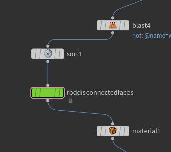
This inserts a ![]() Sort SOP, which sorts the geometry according to the attributes we created above with the
Sort SOP, which sorts the geometry according to the attributes we created above with the ![]() Enumerate SOPs. This way the
Enumerate SOPs. This way the ![]() RBD Disconnected Faces SOP knows which geometry to act on. The Bullet Simulation has scrambled the geometry and this process allows us to sort it.
RBD Disconnected Faces SOP knows which geometry to act on. The Bullet Simulation has scrambled the geometry and this process allows us to sort it.
Now the inside faces of the glass are made non-visible until the relative position exceeds the distance threshold defined in the RBD Disconnected Faces SOP.
Tip
1e-06 means .0000001 (note the six zeros before the 1).
Save to Disk 
After you are happy with the simulation, you will probably want to save it to disk so you are not simulating it live while rendering.
Of course, you can simply cache the simulation to disk using a File SOP or File Cache SOP. However, a more efficient way is to use the ![]() RBD I/O SOP with the “Storage Type” set to “Geometry and Points.” This saves each frame of the simulated points coming out of the RBD Bullet Solver along with one rest frame of the geometry. The single-frame static geometry is then transformed using the light-weight points. It makes for a significant disk I/O improvement both in terms of storage space as well as viewport performance. Loading packed prims on every frame isn’t particularly efficient.
RBD I/O SOP with the “Storage Type” set to “Geometry and Points.” This saves each frame of the simulated points coming out of the RBD Bullet Solver along with one rest frame of the geometry. The single-frame static geometry is then transformed using the light-weight points. It makes for a significant disk I/O improvement both in terms of storage space as well as viewport performance. Loading packed prims on every frame isn’t particularly efficient.
Debugging 
Issue |
Cause |
|---|---|
Parts of the simulation are acting strangely, flipping, or floating in the air. |
About 99% of issues with sims “freaking out” are due to missing or duplicated |
The proxy sim looks fine but the hi-rez sim does not match. |
See above. |
Next Steps 
It is now time to try to do this for yourself. Click the Reset button and try to create the simulation from scratch. Here are some tips:
-
Have another Houdini open with the finished version of this tutorial in it for reference.
-
Replace the hitter sphere with another object.
-
Add another wall or some kind of decoration on the existing wall or window.
-
Try turning ON the clustering option in the RBD Material Fracture SOP for the wood material.
-
Add some debris to this simulation using the
 Debris Tools.
 -
Add some dust to this simulation using the Pyro tools.
-
Simulations look best if they have the following characteristics:
-
A good distribution of sizes according to the power law. That is, there should not be a completely random distribution of sizes. There would probably be a LOT of little pieces, a few medium pieces, and only a couple of bigger pieces.
-
A few remaining pieces that are easily identifiable. For example, “This is obviously a section of the wall.”
-
A “cascading chain of destruction.” That is, everything should not happen on one frame. The destruction should happen over time, and continue after the initial blast. Let the viewer enjoy it.
-
Detail, scale, and variation. Give the viewer something to look at in each section of the frame and during each moment.
Be especially careful to avoid the “shatters like glass” look. This is a common error in beginner’s simulations. Your simulation should look like it is made of various materials with different strengths and breaking thresholds.
-