| On this page |
Overview 
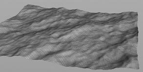
This tool creates a guided FLIP simulation of a thin particle layer on top of an ocean surface. The particles are initialized with ocean velocities. The ocean surface at a specified depth acts as a collision layer underneath the particles, allowing the particles to closely match the ocean waves. A boundary layer of particles suppresses reflections at the edge of the tank, contributes ocean velocities back to the simulation, and maintains the water volume level to match the ocean. The FLIP Simulation uses a guiding volume approach to maintain ocean velocities through the simulation.
The thickness of the thin layer will determine how closely the simulation matches the underlying ocean surface. The thickness will also determine how well the simulation can capture motion below the surface such as wakes and vortices.
The Guided Ocean Layer can be a static simulation or can follow a moving object through the ocean.
The ![]() Ocean Spectrum node allows you to shape the initial frame of your simulated ocean, and
Ocean Spectrum node allows you to shape the initial frame of your simulated ocean, and ![]() Ocean Source controls the outputs.
Ocean Source controls the outputs.
Tip
For more information, see the differences between ocean tank types help page.
Using Guided Ocean Layer 
-
Click the
 Guided Ocean Layer tool on the Oceans tab to create a tank.
 -
Select an animated object to follow and press Enter to confirm your selection. If no object is selected, you will be prompted to place a static tank.
Note
The layer for free fluid particles between the ocean surface and the guiding volume is controlled by the Layer Size parameter in the ![]() Ocean Source SOP.
Ocean Source SOP.
For specific parameter information, see the ![]() Ocean Source help page.
Ocean Source help page.
Changing the look of your ocean 
| To... | Do this |
|---|---|
|
Set the height of the wave |
Navigate to the This value is multiplied by the Speed parameter on the Wind tab.
|
|
Set the direction of the waves |
Navigate to the This controls how many frequencies are moving in the same direction as the wind. Increasing this value will cause more frequencies to travel in the same direction, which is useful for creating shoreline effects. You can also try increasing the Directional Movement parameter. This will dampen the waves moving in the opposite direction of the wind, leaving only the ones moving in the same direction.
|
|
Control the height of the peak |
Navigate to the Increasing this parameter creates sharp peaks on waves. However, if this value is too high waves, may invert on themselves.
|
|
Add more detail to your ocean |
Increase the Resolution Exponent parameter on the Note The Resolution Exponent parameter will not only determine the quality of your ocean, but also the size of the texture maps that you will eventually write out.
|
|
Create a large ocean |
Use the |
Understanding the network of nodes 
There are three important layers to focus on when creating your ocean. First create the ocean, next add whitewater, and finally add specularity for the whitewater.
Tip
Disable all whitewater nodes at the OBJ level while you work on your ocean, then disable the ocean nodes while you work on your whitewater.
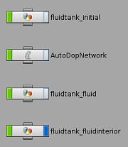
The first set of nodes control the ocean itself.
-
fluidtank_initialcontrols the first frame of your simulation. This is where you can shape the initial frame of your tank with Ocean Spectrum and control the outputs with
  Ocean Source. This includes the size of your tank, the depth of the water etc.
 -
AutoDopNetworkcontrols the simulation of your tank. This is where you will find the FLIP Object and
  FLIP Solver. The FLIP simulation will contain
  Volume Source DOPs to sink and source the boundary layer particles, and a
  Gas Guiding Volume DOP to add ocean velocities to the simulation. Note, the
  Beach Tank shelf tool uses
  POP Advect By Volumes to inject ocean velocities.
 -
fluidtank_fluidis the result of #1 and #2 combined, and is where the results are rendered. After the simulation is done, this node collects the fluid particles, sets up a material, creates some nodes for surfacing to finish the effect. -
fluidtank_interioris also used for rendering, and for creating the volumetric effect that one of the shaders applies to the interior of the fluid. It controls the volume beneath the surface, such as how cloudy or murky the water will appear.
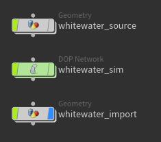
The next set of nodes are to control the whitewater.
Note
To add whitewater to your simulation, use the ![]()
![]() Whitewater tool on the Oceans shelf.
Whitewater tool on the Oceans shelf.
-
whitewater_sourceis where the spray and foam is coming from. -
whitewater_simis where the whitewater simulated. This is where you can modify the animation. -
import_whitewateris the result of #1 and #2 combined.
For more information see How to animate a wave tank with whitewater.
Note
If you build a completely procedural ocean (using the ![]() Large Ocean or
Large Ocean or ![]() Small Ocean shelf tools, for example), the
Small Ocean shelf tools, for example), the ![]() Ocean Foam SOP is used.
Ocean Foam SOP is used.
Understanding the extended ocean surface nodes 
The ![]() Guided Ocean Layer and
Guided Ocean Layer and ![]() Ocean Flat Tank tools also create a network for rendering an “extended” fluid surface that can stretch to the horizon and be rendered with ocean displacement to provide a seamless integration between a FLIP simulation and the surrounding source ocean.
Ocean Flat Tank tools also create a network for rendering an “extended” fluid surface that can stretch to the horizon and be rendered with ocean displacement to provide a seamless integration between a FLIP simulation and the surrounding source ocean.
-
The
 Particle Fluid Surface node (called
 particlefluidsurface1) creates the extended FLIP mesh. The settings on the Flattening tab of this node will flatten the fluid simulation near the edges of the simulation area, and extrude the edges of the polygonal mesh outwards to form an extended flat surface. This flat area surrounding the simulation is then rendered with ocean displacement. -
The two Particle Fluid Mask nodes (called
particlefluidmask1andhifrequency_mask) will create masks on the input ocean spectra that limit the render-time ocean displacement to specified areas of the simulation, usually where there is little velocity, vorticity, or splash height in the fluid. These nodes also blend in ocean displacement around the edges of the simulation bounding box to match the flattening applied while surfacing. Thehifrequency_masknode additionally filters the incoming ocean spectra to remove all but the highest-frequency waves, usually so these can be applied to the simulated FLIP mesh and allow it to better integrate with the surrounding ocean. -
The
surface_previewnode is a fast preview of the FLIP simulation that then samples the created mask to allow visualization of the ocean contribution using a viewport visualizer on themaskattribute. Theoceanevaluate1node applies ocean displacements to that preview based on the calculated masks. -
The
split_spectra_masksnode will separate out the static ocean spectra from the time-dependent masks created by the masking nodes. They are cached to two different sets of files to take advantage of the Ocean Surface material’s ability to have separate spectra and mask inputs.
Tips for improving the look of your water 
-
The defaults for the tank will create a low res simulation, which makes it easy to animate. However, to create a nice looking render, you will need to change some of the defaults. For example, you will need to increase the number of particles in your scene. Decreasing the Particle Separation parameter to about
0.03will create a simulation with approximately 30 million particles. -
Add an environment light to your scene. Water reflects and refracts a lot of the environment around it, so having an environment map in your scene will significantly improve the look.
Tip
In your Environment Map parameter, navigate to the
HFS/houdini/pic/folder and choose the sky fileDOSCH_SKIESV2_${F2}SN_lowres.rat.
| See also |