| On this page |
Overview 
The ![]() Ripple Solver SOP is useful for creating ripples propagating on shallow water surfaces. For example, ripples caused by rain drops or bow waves created by a boat moving through water. It can also be used to generate cartoon-like effects on fabric or skin, pumping/breathing effects, and organic motion. The solver works best on flat geometry, but is also very reliable on 3D objects.
Ripple Solver SOP is useful for creating ripples propagating on shallow water surfaces. For example, ripples caused by rain drops or bow waves created by a boat moving through water. It can also be used to generate cartoon-like effects on fabric or skin, pumping/breathing effects, and organic motion. The solver works best on flat geometry, but is also very reliable on 3D objects.
There are two general approaches for creating ripples. However, it’s also possible to combine both approaches.
-
One method uses the difference between an object’s original rest (first node input) and deformed (second node input) states. When using this method, the object’s topology must not change: the number of points, vertices, and faces have to be identical for the object’s rest and deformed states.
-
Another method for creating ripples is to connect one or more collision objects to the solver’s third input. The object’s position determines the ripples' originating point. Collision objects create impressions on the rest geometry. The object’s scale also controls the size of the ripples' center. Collision objects can be static, moving, or deforming.
The node’s first input is mandatory. If the second input is empty, because rest and deformed states are identical, the solver tries to use the object from the first input. In this case you will see a warning.
Note
Currently, collision objects only create ripples, but waves aren’t reflected from their surface to create complex patterns.
The ripple solver is similar to the ![]() Shallow Water Solver SOP. However, the Shallow Water Solver is based on heightfields, while the Ripple Solver uses a geometry approach. It is important to note that, when using the Ripple Solver, collision objects can only create impressions. Bulged surfaces, for example from a submarine traveling below the water surface, aren’t possible.
Shallow Water Solver SOP. However, the Shallow Water Solver is based on heightfields, while the Ripple Solver uses a geometry approach. It is important to note that, when using the Ripple Solver, collision objects can only create impressions. Bulged surfaces, for example from a submarine traveling below the water surface, aren’t possible.
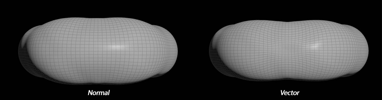
You can also choose from two Wave type options: Normal and Vector. With Normal, the points are only displaced along the object’s normals. Additionally, the solver’s displacement point attribute is scalar and stores a point’s current distance from the rest position. With Vector, there’s no such restriction and the displacement attribute is a vector. To see the displacement attribute’s value, open the solver’s Output tab and turn on Displacement. You can find the values in the Geometry Spreadsheet.
Example: basic ripples 
The following example explains how to create ripples traveling over a ![]() Torus SOP. The ripple solver creates waves from the difference between an object’s rest and deformed states. The distance between these states determines the wave height.
Torus SOP. The ripple solver creates waves from the difference between an object’s rest and deformed states. The distance between these states determines the wave height.
Object 
To get a smooth wave surface, the object needs a certain amount of detail: the more points/polygons it has, the better the waves.
-
At the obj level, put down a Torus and double-click it to dive into the node.
-
Select the torus and set Rows to
60and Columns to120to get enough resolution.
Point group 
For this step you’ll create a point selection and displace the points to determine the waves' origin. Before you start, hover the mouse cursor over the viewport and press 3 to switch to Front mode. You might also want to press W the turn on a shaded mode. This will help you to select the points.
-
Add a Group SOP and connect its input with the output of the Torus node.
-
Go to Group Name and replace the default entry with
wave_origin(or any other name). -
Change the Group Type to Points, and click the
 icon beside the Base Group parameter.
 -
⇧ Shift-click the points you want to select or draw a rectangle around the with the mouse.
Note that the selection tool will also select hidden points form the rear surfaces. If you want to get rid off them, move the mouse over the viewport again and press 0 for the Perspective mode. To deselect a point, ⌃ Ctrl-click it or draw a rectangle around a group of points. Press Enter to confirm your selection and the point indices will appear in the Base Group parameter.
The pattern could be a cross-shaped selection as shown below.

Displacement 
-
Add a
 Soft Peak SOP and connect it to the Group SOP.
 -
On the Group parameter, type
wave_originto restrict the node’s effect to the previously selected points. -
Set Distance to
0.15to displace the selected points. This is important because without initial deformations, nothing will happen when you press play. -
Turn off Translate Along Lead Normals to get a smooth surface.
-
The Soft Radius parameters flattens the polygons around the point selection and turns the cross-shaped selection into a bubble. For hard edges, decrease the value.
What you have now is an original rest state and a deformed version with displaced points.
Ripples 
The solver calculates the difference between both versions to create the ripples.
-
Add a
 Ripple Solver SOP and connect its first input with the Torus SOP’s output.
 -
Connect the solver’s second input (Deformed Geometry) with the Soft Peak SOP’s output.
-
On the playbar, click the
 Play forward icon to start a first simulation.
Here is what you can get with the Ripple Solver’s default settings. The colors represent the displacement values.
Ripple speed 
On the Ripple Solver’s Setup tab you can find two parameters for controlling the ripples' speed: Wave Speed and Rest Spring. Wave Speed defines how fast the ripples travel from point to point. Rest Spring is a force that tries to pull the displaced points towards their rest position. When Wave Speed is 0 and Rest Spring is set to 1 (or greater), it will create a back and forth movement, similar to a pumping or breathing effect. Increasing the Rest Spring value to 10 or higher will create more up and down cycles.
Conservation doesn’t contribute to the ripples' speed, but lets the waves fade out over time. A value of 1, will result in the ripples keeping their entire energy and move infinitely. Values less than 1 will cause the waves to lose energy. For example, a value of 0.7 will cause the waves to lose 30% of their initial energy after one second. A value of 0.2, will cause the waves to lose 80%.
Substeps 
Substeps define the simulation’s accuracy. The Ripple Solver’s substeps are adaptive. The solver calculates how many substeps are required to keep the simulation stable. The actual number lies between the Min Substeps and Max Substeps. One of the first things you can do when you observe stability issues is increase the solver’s Min Substeps. If the solver requires more maximum substeps than adjusted, then Wave Speed and Rest Spring will be clamped internally to maintain stability.
To check if speed and spring force are clamped, go to the solver’s Output tab and turn on Substep Clamped. Open the Geometry Spreadsheet and simulate. If the substepclamped point attribute is 1, then speed and spring force are clamped.
Thickness 
The thickness attribute is positive number that indicates how thick the geometry is at this point. It is used to clamp the height of waves at each point and to determine the amount of distortion due to collisions. If this attribute is not present, the point thickness is determined by settings on the Thickness tab.
Clamping 
The parameters on the Clamping tab are associated with thickness. Clamping means that all displacement values greater than Thickness are cut off. Cutting off the values can create hard edges. To restore a smooth and more organic look, use Soft Clamp Falloff.
-
To see the effect of clamping, turn off Enable Clamping and set Soft Clamp Falloff to
0. -
Additionally, set Thickness to
0.1. The actual displacement determined in the Soft Peak SOP’s Distance value is0.25. When you look at the viewport, the object looks as before. If you turn on Enable Clamping again, and you will see that the bubble’s shape has changed. -
To restore the smooth look, increase Soft Clamp to
1and Soft Clamp Falloff to2.
Example: rain drops 
This example demonstrates how to use the Ripple Solver SOP’s third input to create raindrops. The idea is to scatter several small spheres over a plane. These spheres act as seeds for small waves. Time-based expressions and noise attributes create a natural distribution.
Water and rain drops 
The water surface in this project is a high-resolution grid to get enough details. Then you’ll randomly place spheres with variable size on the grid. The spheres will act as colliders and the “impact” creates the waves.
-
At the obj level, put down a
 Grid SOP and double-click it to dive into the node.
 -
Select the grid node and set the Size parameters (width and height) to
7.5. -
Increase Rows and Columns to
500to get enough resolution for small ripples. -
Add a
 Sphere SOP and decrease Uniform Scale to
 0.1. This object will be instanced to create the raindrops. -
Play down a
 Scatter SOP and connect its input with the Grid SOP’s output.
 -
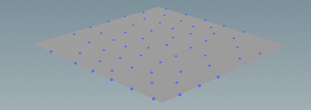
On the scatter node, change Force Total Count to
7. This parameter specifies the number of sphere instances. To introduce new spheres with each frame and delete the previous objects, change Global Seed to$F. This expression changes the spheres' distribution over time. However, the number of new spheres per frame remains constant.
When you turn on the scatter node’s blue Display/Render flag, you should see seven black dots in the viewport. Drag the timeline slider to see how the points' distribution changes over times.
Ripples from instances 
To create the instances, copy the spheres onto the scatter points. Here’s a preview of the complete network.

-
Add a
 Copy to Points SOP and connect its first input with the sphere’s output. The second input is linked to the grid’s output.
 -
Put down a
Ripple Solver SOP.Connect its first and second input with the output of the grid. The third input goes to the output of the Copy to Points SOP. -
To dampen the ripples and make them vanish over times, change Conservation to
0.3on the Setup tab. -
Click the
Play forward button to start the simulation.
You can see the sphere instances as blue wireframe objects. The solver recognizes the spheres as collision objects and creates waves around them. When you render the scene, the blue instances won’t be considered. In the image below the number of rain drops was increased for illustration purposes.
Masking 
To change the uniform look of the rain drops' distribution you can apply a dynamic mask. The mask spares out certain areas and you get zones with more or less drops.
-
Add an
 Attribute Noise SOP and place it between the grid and scatter SOPs to connect it.
 -
Beside the Attribute Names parameter, turn off the Y and Z buttons to keep only the
Cdattribute’s red color. -
From the Range Values dropdown menu, choose Zero Centered.
-
Change the Offset parameter value to
$F. Again. this expression uses the current frame to change the noise pattern over time. -
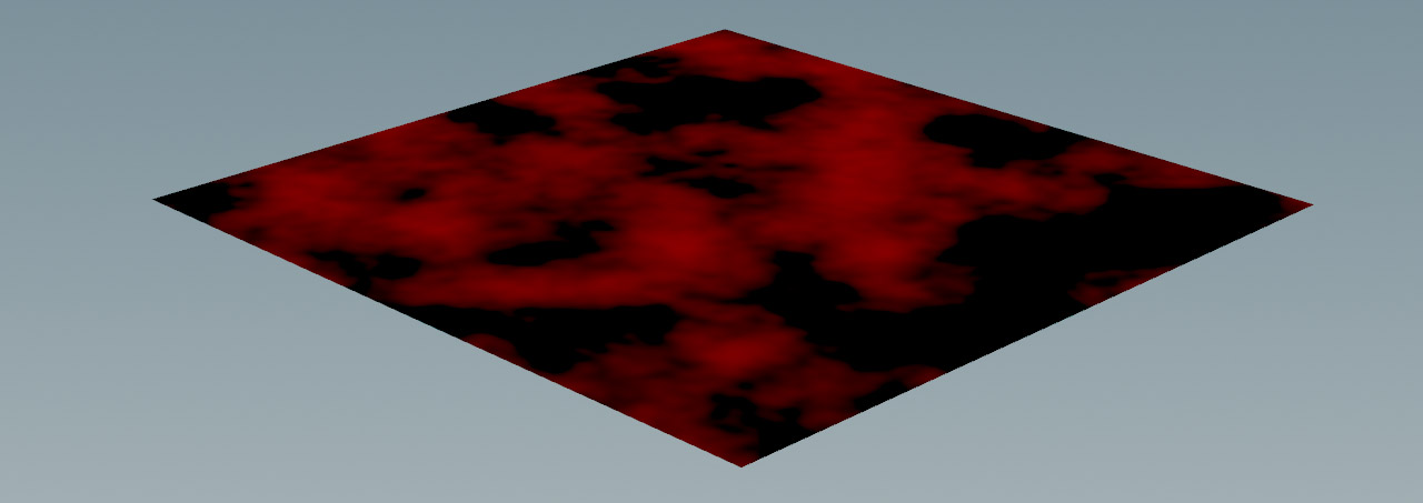
On the Scatter SOP, turn on Density Attribute and replace
densitywithCd. The red parts of the noise pattern will determine where the scatterer creates rain drops. -
To delete the colors after the creation of the instances, put down an
 Attribute Delete SOP and place it between the copy to point and solver nodes to connect it.
 -
Go to Point Attributes and enter
Cd. -
Press the Play forward button to simulate.
Here’s a screenshot from the color mask.
Randomizing scale 
You can also randomize the size of the drops for even more realism.
-
Add an
 Attribute Randomize SOP and place it between the attribute noise and copy nodes to connect it.
 -
Under Attribute Name replace
Cdwithpscale. -
On the Distribution tab, choose Two Values from the Distribution dropdown menu to define the drops' minimum and maximum size.
-
Set Dimensions to
1, becausepscaleis a scalar. -
For Value A, enter
0.6. The Value A/B parameters are multiplied with the sphere’s current scale to get the actual value. -
Simulate again.
How to 
| To... | Do this |
|---|---|
|
Fade out ripples |
By default, ripples don’t lose energy and virtually propagate forever. To make the ripples fade out, open the solver’s Setup tab and decrease Conservation. A value of |
|
Change ripple speed |
The Wave Speed parameter is located in the Setup tab. With higher Rest Spring you create more up and down cycles. More cycles per time unit also mean faster ripples. |
|
Fix instabilities |
Increasing substeps is a common method to fix instabilities. On the Simulation tab, first try increasing Min Substeps. If this doesn’t fix the issue, also increase Max Substeps. Another way to get rid of instabilities and chaotic surface structures is to remove energy from the ripples. You can decrease Wave Speed on the Setup tab, and make the ripples fade out with lower Conservation values. |
|
Increase quality |
Lowering the CFL Condition parameter will produce higher quality results, but will be slower to compute. The default is 1 and produces good results, so it rarely needs to be changed |
|
Prevent geometry from folding in on itself |
Turn on Enable Clamping so that displacement on a point does not go beyond the thickness of that point. You can also use the Soft Clamp Falloff parameter to smooth the transition when displacement gets close to thickness at a point. |
|
Use objects as ripple sources |
The Ripple Solver SOP’s third input accepts objects and uses their position and size to create impact ripples. For a complete workflow guide, see the rain drops example. |