| On this page |
Note
This guide requires a basic knowledge about heightfields and the Shallow Water Solver. Some of the examples in this chapter are also based on the heightfield and solver settings from the introduction to the Shallow Water Solver to become familiar with fundamental setups and workflows.
When you look at the ![]() Shallow Water Solver SOP’s Output tab, you can see three parameters that let you store velocity, acceleration and vorticity data as layers. You can use the information for visualizing differences in speed or vorticity, but also for trailing effects. Another field of application is to use fields to drive simulations.
Shallow Water Solver SOP’s Output tab, you can see three parameters that let you store velocity, acceleration and vorticity data as layers. You can use the information for visualizing differences in speed or vorticity, but also for trailing effects. Another field of application is to use fields to drive simulations.
Velocity 
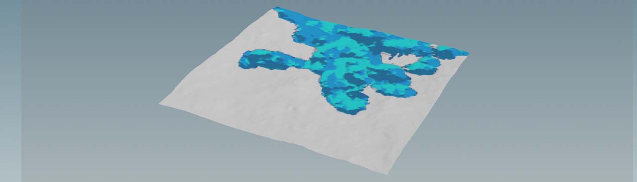
Velocity is turned on by default and you can directly map the different velocities to the simulation: From the Visualization dropdown, choose Color Water by Layer. If you already went through the introduction to the Shallow Water Solver, you know that this option adds a turquoise-blue gradient that represents the water’s velocities. The Visualization parameters let you control the gradient’s color distribution.
For more information, open the Geometry Spreadsheet and click the ![]() Primitives button. There you’ll see that there’s no combined
Primitives button. There you’ll see that there’s no combined velocity layer, but you have individual vel.x, vel.y and vel.z layers instead. It’s also important to know that vel.y is always zero, because heightfields are 2D grids without a physical height.
Vorticity 
The vorticity layer stores the local rotational motion at each point, with larger absolute values indicating faster spinning. Positive vorticity values signal that rotation is in the counter-clockwise direction when viewed from above; negative values indicate a clockwise rotation.
The Shallow Water Solver does not provide any built-in features to visualize vorticity and you need a custom solution.
Acceleration 
Acceleration is the rate at which an object’s velocity changes over time. It can mean speeding up, slowing down, or changing direction. Like velcoity, the acceleration layer consists of three components: accel.x, accel.y and accel.z, but again, only the X and Z components are relevant. There’s no out-of-the-box feature for displaying this layer and you need a custom solution.
Force 
The solver’s Binding tab provides an empty Force Mask Layer. You can create a custom, animated mask and connect it to the slot. The solver will use the mask values to push and displace the water.
Tip
There’s an example further down that explains how to create a pulsating radial force layer.
Visualization: Layers 
Houdini’s heightfields provide a ![]() HeightField Visualize SOP that lets you define custom colors for up to nine layers. A common application with this node is texturing.
HeightField Visualize SOP that lets you define custom colors for up to nine layers. A common application with this node is texturing.
The visualize node is typically the last node of your network, because only then you can be sure that all layers will be available. The node’s usage is straightforward:
-
On the Material section you can see a Height Ramp. The gradient tints the terrain according to the values of the
heightlayer. You can click Compute Range to map the entire range of gradient colors to the terrain. When you click the Presets button, you choose from various predefined color ramps.
 -
Each of the nine Layer parameters has an associated dropdown menu that list the entire range of existing layers. Choose a layer or type its name to an empty parameter field. Then, define a Color. The layer will be displayed with the chosen color.
Note
The layer numbers also indicate how layers are stacked. Imagine the floowing example where assign vel.x and vel.z to Layer 1 and Layer 2, but water to Layer 3. In this scenario, the water layer will cover the velocity layer and they're no longer visible. To get a correct result, assing water to Layer 1.
Visualization: Trails 
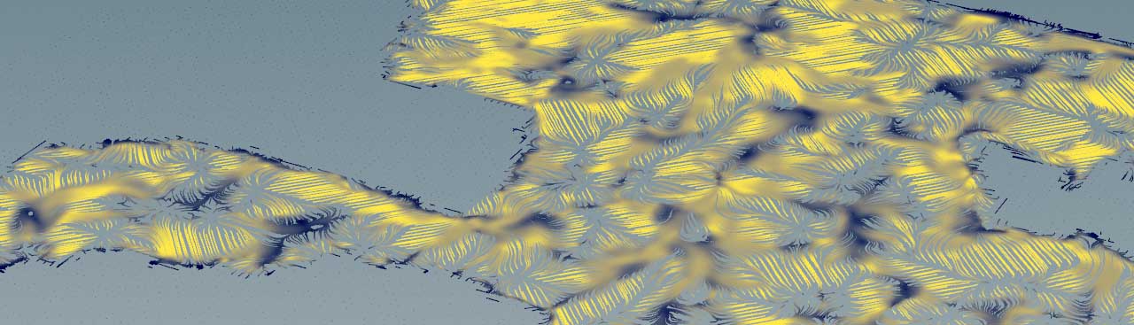
You can visualize the information from the solver’s layers to create trails with mesmerizing swirling and curling effects. As the name indicates, the node was made to show volumes, but a heightfield is a 2D grid. The Y coordinate is always zero and this is the reason why you will also only see a flat representation.
-
Add a
 Volume Trail SOP to the network and connect its second input with the output of the solver.
 -
Lay down a
 Grid SOP and connect its output with fist input of the solver.
 -
Adjust the grid’s Size parameters so that they match the Size values of the
 HeightField SOP. For example, if the heightfield is 100 m by 100 m, the Size values for both nodes are
 100as well. -
The grid’s Rows and Columns parameters define the resolution of the trails. It’s not possible to give exact values here, because they depend on several factors.
-
On the trail node, go to Velocity Volumes and enter the name of the field you want to visualize. You can also choose an entry from the parameter’s associated dropdown menu.
-
Then, adjust Trail Length. Longer trails take longer to be drawn and will also create a denser “map”.
If the shallow water simulation is cached, you can move the Playbar head or press the ![]() Play button to see the trails in motion.
Play button to see the trails in motion.
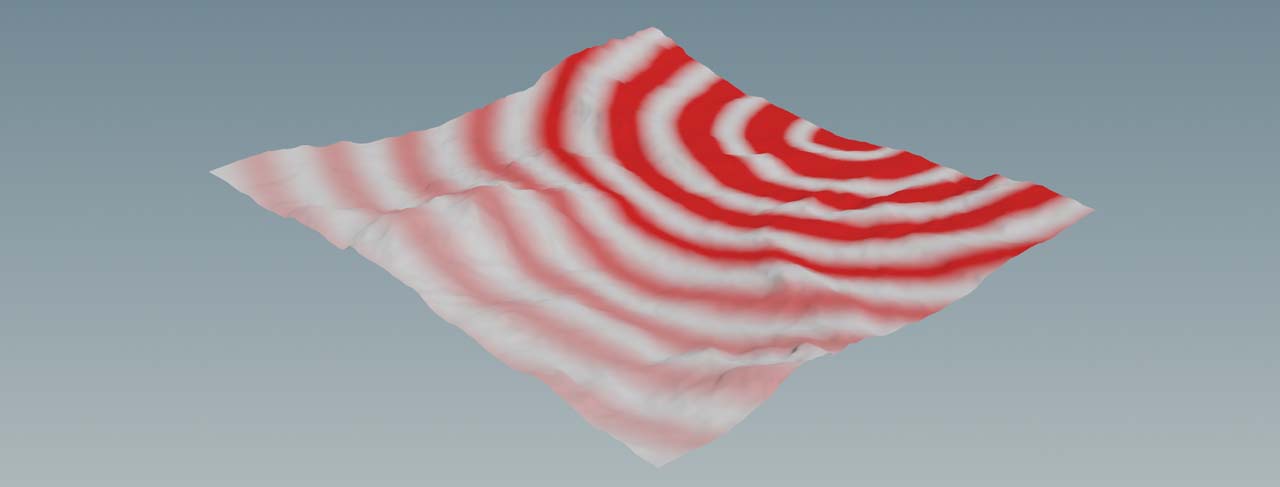
Creating a force field 
Houdini offers a wide range of methods to create custom fields. However, the various techniques have one thing in common if you want to use them with the Shallow Water Solver: The force must be converted into a mask. The following example illustrates how to draw an animated radial mask that pushes the water away from the mask’s center.
Terrain 
To get a better view of the force, you should make the terrain smaller. For the HeightField SOP’s Size parameters, enter 100, 100. To get more detail, set Grid Spacing to 0.5 - this will also be the value for the solver’s Voxel Size Scale parameter. Most probably you have to decrease the Amplitude and Element Size parameters of the ![]() HeightField Noise SOP to get more surface detail.
HeightField Noise SOP to get more surface detail.
-
You can modify the terrain to your liking, but don’t make it too high, because the water should be able to propagate over the landscape.
-
You also need a
sourcelayer to determine where the water will be created. The steps to create this layer are explained on the Shallow Water Solver page.
VEX script 
The idea is to use a VEX script that creates propagating concentric rings and converts them into a mask. Several custom parameters give you full control over the resulting force. To apply a script to a terrain you need a ![]() HeightField Wrangle SOP. In your network, place the wrangle directly before the solver and connect its first input.
HeightField Wrangle SOP. In your network, place the wrangle directly before the solver and connect its first input.
Then use ⌃ Ctrl + C to copy the script below and paste it with ⌃ Ctrl + V to the wrangle’s VEXpression field. Click the ![]() Creates spare parameter for each unique call of ch() button to add the custom parameters to the wrangle’s parameter set.
Creates spare parameter for each unique call of ch() button to add the custom parameters to the wrangle’s parameter set.
// Parameter section
vector center = chv("center");       // Custom parameter: Wave center
float speed = chf("speed");          // Custom parameter: Wave speed
float frequency = chf("frequency");  // Custom parameter: Wave frequency
float amplitude = chf("amplitude");  // Custom parameter: Mask strength (= force strength)
float falloff = chf("falloff");      // Custom parameter: Strength attenuation factor
float time = @Time;                  // Current simulation time

// Current heightfield position
vector pos = @P;

// Distance of the current position to the wave center
float dist = distance(pos, center);

// Wave creation
float wave = sin(dist * frequency - time * speed);

// Remap wave to a [0,1] range and scale the result with the waves' strength
float mask = fit(wave, -1, 1, 0, 1) * amplitude;

// Optional: Wave strength decreases with increasing distance from the center
mask *= exp(-dist * falloff);

// Write the result to the heightfield's @mask layer
@mask = mask;
Parameters 
The following table gives you an idea what the custom parameters do. The actual values strongly depend on the size of the terrain. The settings below were tested for a terrain size of 100 m by 100 m. To see the effect of your changes, turn on the wrangle’s blue Display/Render flag.
| Parameter | Description |
|---|---|
| Center |
Defines the center of the waves. Consider that heightfields are 2D and you’ll only need the X and Z values. Place the center near or inside the painted source mask. This makes sure that waves can influence the water. You can use positive and negative values. For example, in a 100 m by 100 m terrain, the left edge is at X = -50, the lower edge is at Z = 50.
|
| Speed |
The propagation speed of the waves. Start with values between 2 and 5.
|
| Frequency |
This parameter defines the number of waves/rings. With smaller values you’ll get a denser pattern. Higher settings create thicker rings. Try to stay between 0.2 and 1.
|
| Amplitude |
This is the strength of the mask. The mask values are then converted into a force. For this example scene start with values between 1 and 5. Very high Amplitude values might lead to instabilities.
|
| Falloff |
You can make the waves fade out with increasing distance from the center. This parameter is very sensitive and you should start with small values around 0.02.
|
Layer creation 
The next step is to convert the mask into a force layer you can use to drive simulation. As with the source layer, you also need a ![]() HeightField Copy Layer SOP. Place the node between wrangle and solver to connect it and set its Destination to
HeightField Copy Layer SOP. Place the node between wrangle and solver to connect it and set its Destination to force.
A ![]() HeightField Mask Clear SOP downstream of the copy node resets the circle mask. For Layer 1, enter
HeightField Mask Clear SOP downstream of the copy node resets the circle mask. For Layer 1, enter mask.
Solver adjustments 
You also need some adjustments on the solver. While most parameters on the Setup tab strongly depend on the shape and size of your terrain, there are a few settings you must consider:
-
On the Setup tab, go to the Constraint Updates section. From the Forces Frequency dropdown menu, choose Every Substep. This option will apply the values of the
forcelayer with every simulation substep. You can also apply the force at every frame, but substeps tend to create a smoother result - even if this method takes longer to simulate. -
On the Bindings tab, go to Force Mask Layer and enter
forceto establish a connection between the solver and the new layer.
On the Simulation tab, adjust Voxel Size Scale. For this example with a 100 m by 100 m terrain, a value of 0.5 was used, but you might want to enter a different value. Also on the Simulation tab, you can increase Cache Memory (MB) to cache the result to your computer’s RAM for fast playback.
When you simulate, you should see how the force pushes the water and creates bow-shaped waves as in the time-lapse video below.