| On this page |
As a 3D artist you most probably know the concept of displacement maps, where color information is translated into height information. A typical application for displacement maps are ocean waves, digital elevation models or the creation of complex structures from a simple base geometry.
In contrast to bump maps, where the normal vector is altered to achieve the visual impression of irregularities, displacement maps create actual geometry. Heightfields, however, consist of volumetric data and the map’s height information is stored in the base grid’s points. When you use displacement maps, you have several ruling factors that determine the quality of your terrain. The most obvious parameters are grid resolution and map resolution. A 2K map for a small ground segment with sand and gravel is normally not suited for a huge terrain. And a terrain with grid points every 2 m will not show as many detail as a model with a point distance of 5 cm.
Another aspect is the used file format. You typically differentiate between 8-bit formats, and EXR or TIFF files with 16 or 32 bit. The more information your file stores, the better the resulting terrain. With 8-bit files you might observe banding or other patterns, caused by insufficient color information. 32-bit images create smoother surfaces. Anyway, for distant areas or ground planes covered with debris or grass, 8-bit images are often enough.
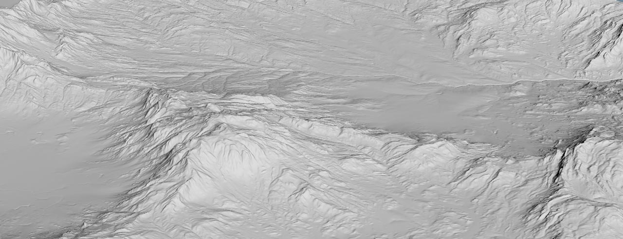
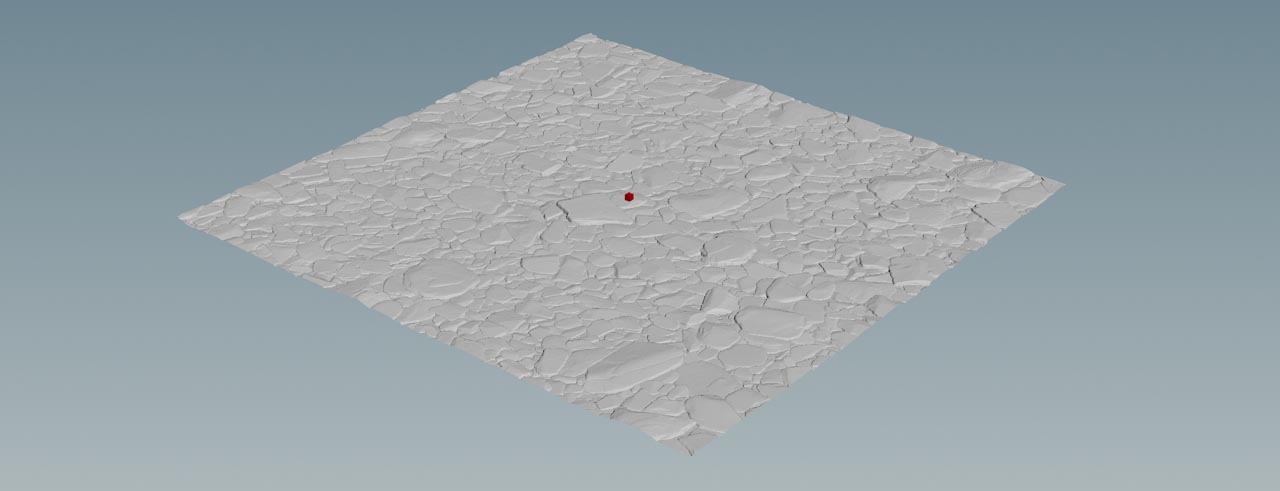
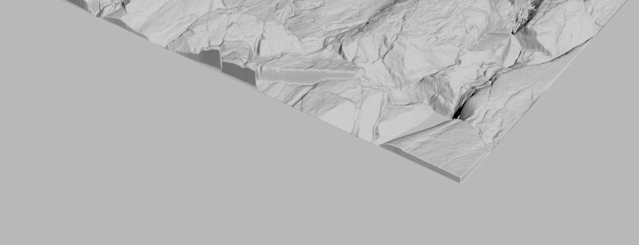
Finally, the surface’s original scale also plays an important role. For example, a displacement map from a small section of a landscape doesn’t look good, when you stretch it over an entire terrain. On the first look, the landscape below appears to be correct, because it has enough resolution. However, the original size of the displacement map is just 2 m by 2 m. When you consider that the map’s features are magnified by a factor of 500, the image starts to look out of scale. The edge length of the red box in the middle is 10 m.
Note
You can use maps in two ways: as a height layer or a mask layer. The latter option is discussed separately on the Masks from images page.
Basic setup 
In order to use displacement maps you need a basic heightfield grid. The setup, described here, will be the basis for all following considerations.
-
On the obj level, press ⇥ Tab to open the tab menu. From there, create a
 Geometry OBJ node. Double-click the new node to dive inside.
 -
Now add a
 HeightField SOP. The map will be projected onto this base grid.
 -
Change Size to
4, 4to create a small area that will serve as a ground. -
Decrease Grid Spacing to
0.002. This value determines the distance between two grid points and lets you see even finest structures. The resulting grid consists of 8,000,000 voxels.
Loading the map 
A displacement map adds detail to the flat grid. Houdini provides a separate node for loading maps. This node also lets you make several adjustments on the map and the height layer directly. The maps, used in this example, cover an area of 2 m by 2 m.
-
Lay down a
 HeightField File SOP and place it between the already existing nodes from the basic setup to connect it.
 -
Next to File click the
 Open floating file chooser button and load a displacement map. As suggested above, you should use 32-bit EXRs for best results.
Note
With very large maps, you might see an
Image resolution too largeerror on the HeightField File SOP. In this case you can go to the main menu’s Edit entry and choose Preferences ▸ Old Compositor. Then, open the Cooking tab and increase the Resolution Limit parameter. -
What you will get is pale red surface without surface structures. The reason for this look is found in the Layering section. There, you can see that Layer Name is set to
maskand the map is therefore treated as a mask. To create surface structures, change the entry toheight.
Size and height 
The heightfield is now most probably shifted along the positive Y axis and maybe you can also recognize a few surface structures.
-
Go to the Size section. There you can see that the Size parameter’s default value is
1000. This corresponds with the heightfield’s standard dimension of1000. Enter4to restore the map’s original size. The terrain is now centered in the middle and embossed, while the area around the map is completely even.It’s possible to upscale high-res 8K or 16K displacement maps to a certain amount, but don’t overdo things to avoid artifacts or blurred structures. A scaling factor of 1.5 to 2 works in many cases.
-
To flatten the terrain, go to Height ▸ Height Scale. The default of
1is also tied to Houdini’s standard terrain and way too large in relation to the small area. Start with a value around0.1- the actual value depends on the map’s original scale.
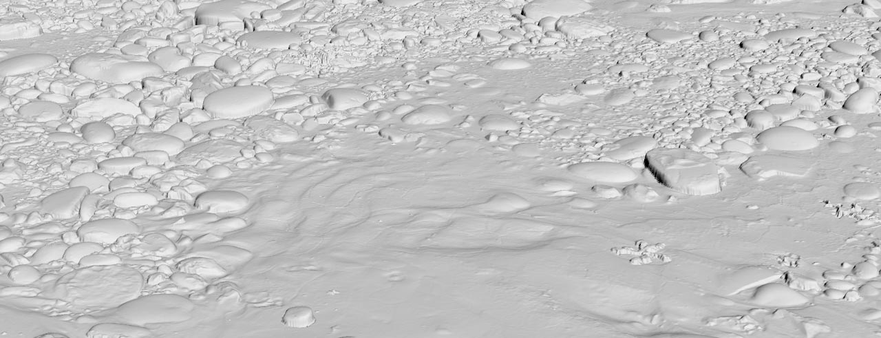
The image shows a section of the pebbles map that was used here.
Layering: Border 
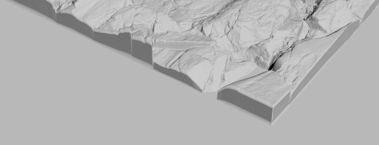
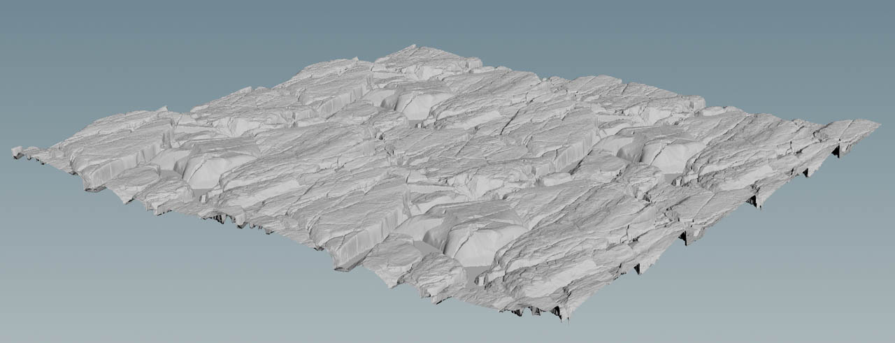
In this example, base grid and map both have a size of 4 m by 4 m. The HeightField File SOP’s Size parameter was also adjusted to 4 and now map and base grid are matching to get the correct scale. What if you load a 2 m x 2 m map and set Size to 2, but leave the grid’s size untouched? This combination creates an embossed effect you can see in the image above.
The Layering section provides some useful tools, e.g. for tiling or how an empty space around a terrain is treated. By default, Border Type is set to Constant. To compensate for the hard edge, you can adjust Border Value. To get a seamless transition from border to terrain, you can use an expression.
-
Right-click on Height Scale. From the menu, choose Copy Parameter.
-
Now, right-click on Border Value and choose Copy Relative References.
-
The input field turns green and now contains an expression. To align border and terrain, change the expression to
ch("heightscale")/2. -
You might have noticed that the entire heightfield was slightly moved upwards. To set the grid back to the scene’s base level, select the HeightField SOP. Right-click on Initial Height and choose again Copy Relative References. This time, the expression is
-ch("../heightfield_file1/heightscale")/2. Now, the grid is at Y=0 again.The idea of relative references is that you have to change a value once only and all referenced parameters will be updated according to the associated formula.
Layering: Tiling 
In fact, tiling also belongs to the “border” topic, but is discussed separately due to its importance. Many displacement maps, esp. those from commercial repositories, are seamless and tileable. So, instead of scaling the map, you can repeat it to cover the entire heightfield area.
-
The HeightField SOP’s Border Type dropdown provides a Repeat option. Choose this entry for tiling the displacement map.
-
The Position section’s parameters let you change the map’s Center and Rotate values.
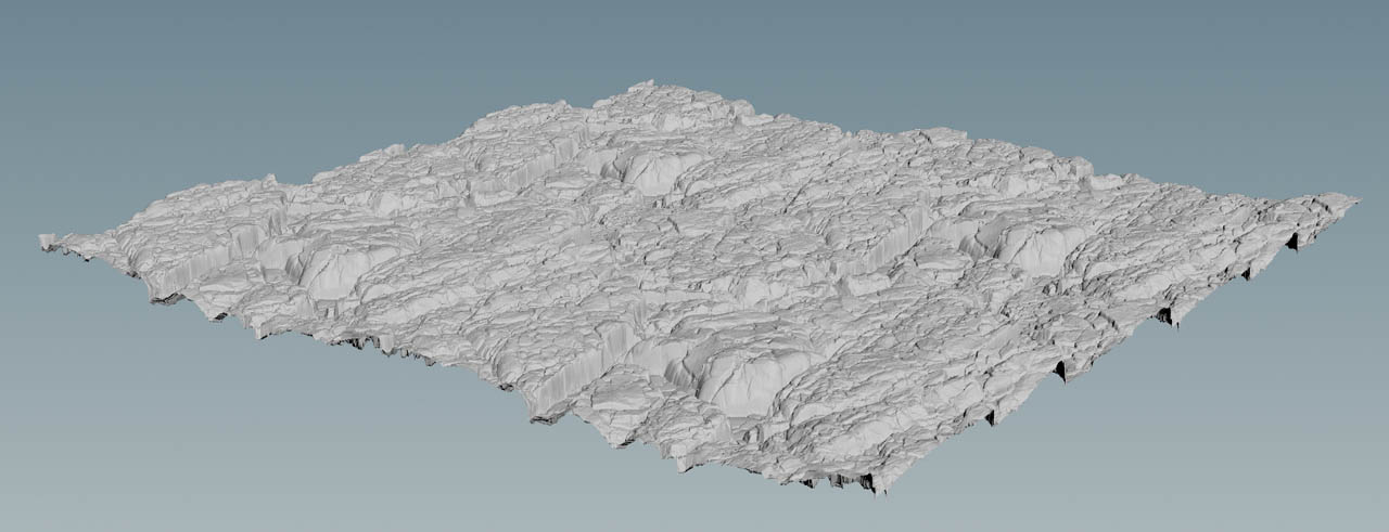
Here you can see the 2 m by 2 m map from the Layering: border chapter above and how it’s repeated to cover the 4 m by 4 m base grid.
Stacking maps 
You're not limited to a single HeightField File SOP, and you can stack several nodes with different maps to create completely new terrains. Displacement maps also merge with other terrain-creating nodes like the ![]() HeightField Noise SOP. The biggest limitation is that, by default, there’s no ready-to-use parameter for blending different maps. Each map contributes equally to the final result.
HeightField Noise SOP. The biggest limitation is that, by default, there’s no ready-to-use parameter for blending different maps. Each map contributes equally to the final result.
If you just want to stack maps, you can chain several HeightField File SOPs and make individual adjustments on them. The only thing to consider is that the Height Scale values of the various maps add up. In a scene with, lets say, three maps and Height Scale values of 0.02, 0.03 and 0.05, the base grid’s Y position will be 0.1. In this example, the HeightField SOP’s Initial Height should be -0.05 to reset the grid to the scene’s origin.
Here you can see the stacking of the two maps used in the previous chapters.
Exporting maps and layers 
The usage of displacement maps isn’t a one-way street, but you can also export your heightfields and bake them into files.
-
Add a
 HeightField Output SOP and connect its input with the output of your network’s last upstream node.
 -
Go to Filename and click the
button to specify output name and directory. The file type is taken from the suffix you enter, e.g. .jpg. -
Turn on Resolution and enter the values for the number of pixels in X and Y direction. Choose values that can be divided by 8, e.g.
256,512,1024or4096. -
Go to the Output Layers section. Next to the color channel parameters, you can see associated dropdown menus. For Red, Green and Red, choose
height. If you also have an alpha mask defined, set Alpha tomask. Otherwise it’s safe to turn off Alpha.Here you're exporting the
heightlayer, but you can choose any other available layer. -
Click the Save to Disk button to write the map to disk.