| On this page |
The Abelian sandpile model is an example for a self-organizing dynamical system and was introduced in 1987. The system applies rules when a sandpile becomes unstable and starts to slide downhill. This process depends on the pile’s slope.
The model is a 2D approach and therefore perfectly suited for Houdini’s heightfields, because a heightfield is also represented as a 2D grid. Once you've formulated the 2D methods, you can update the terrain’s height layer. With the help of a ![]() Solver SOP, you can simulate sand sliding down a pile and eroding its sides.
Solver SOP, you can simulate sand sliding down a pile and eroding its sides.
A basic script that simulates sliding sand requires two ![]() HeightField Wrangle SOPs. The first wrangle iterates over the terrain’s voxels and looks for its top, bottom, left and right neighbors. Then, the script determines the sliding direction with the help of a random function. Lets assume, the solver determined bottom as the voxel that will receive the sand. This means that the bottom voxel’s
HeightField Wrangle SOPs. The first wrangle iterates over the terrain’s voxels and looks for its top, bottom, left and right neighbors. Then, the script determines the sliding direction with the help of a random function. Lets assume, the solver determined bottom as the voxel that will receive the sand. This means that the bottom voxel’s height information must be updated. This, however, is not possible, because VEX doesn’t allow writing into neighbor voxels directly. The solution is to write this information to a separate layer, read out the value in a second wrangle and apply it to the currently processed voxel.
With four cardinal directions, the results may look artificial or mechanical, as if the hillsides were cut into blocks.
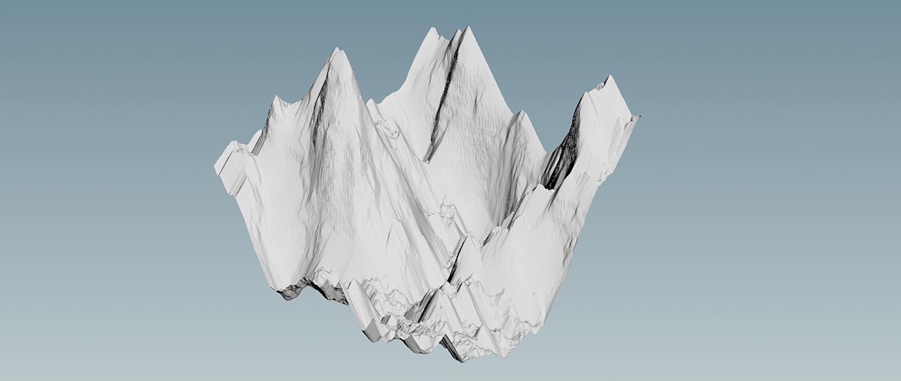
For more natural results, the example script has several additions and extensions:
-
Instead of four directions, the script tests for eight possible directions
-
Sedimentation conserves the eroded sand and fills valleys and depressions
-
To avoid artifacts on the sediment’s surface, the solver uses a basic wind model
Note
The main purpose of this example is to show you a more advanced solution. However, we don’t go into the depths of the Abelian sandpile model, and you can find very good explanations on the internet. The script is also commented and explains what happens in each code block.
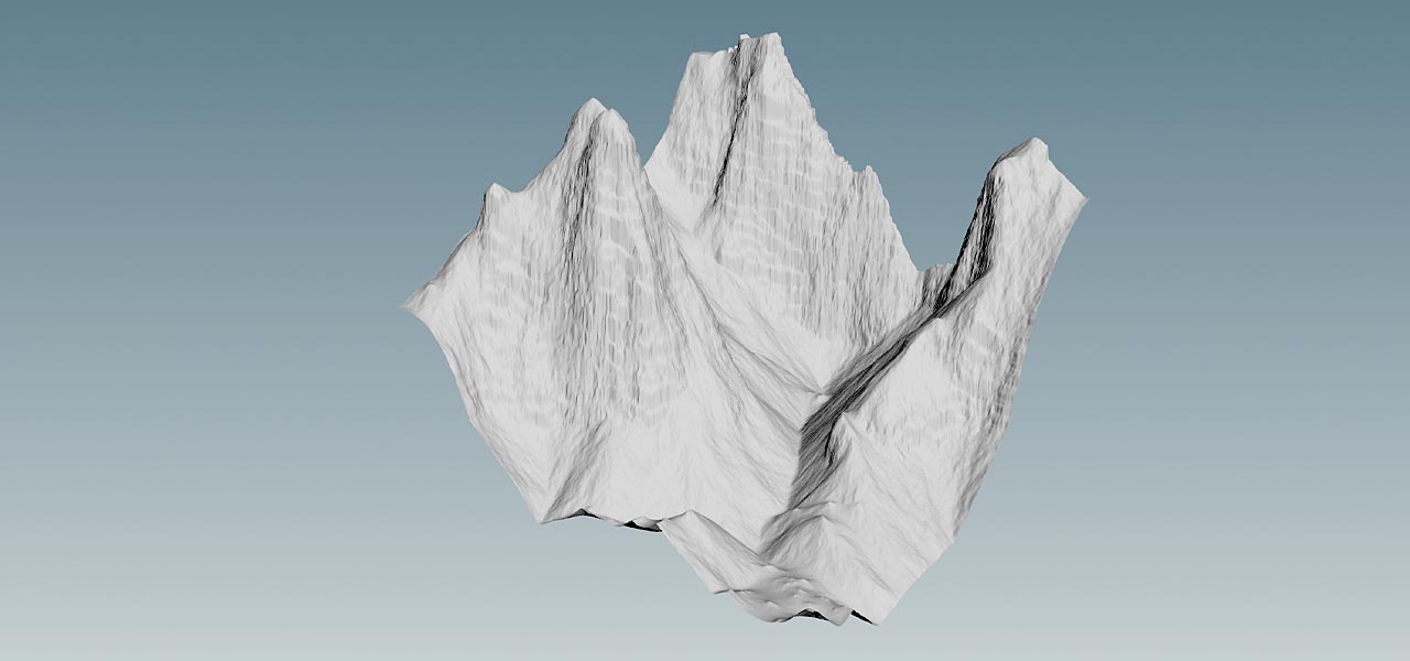
Terrain 
Due to the nature of sandpiles, the terrain should not be too large. A size of approximately 100 m by 100 m is a natural limit, but not a physical barrier. Of course, you can also run the solver on large terrains, but at the cost of longer simulation times and (maybe) unexpected results. With large terrains we also recommend higher Grid Spacing values on the HeightField SOP to cut down simulation times.
The solver will also profit from strong in differences in height. A terrain that is relatively flat by default will hardly show any changes. With steep hills, on the other hand, you can also achieve an interesting terracing effect.
Scene setup 
You start with a basic heightfield. A ![]() HeightField Distort by Noise SOP can help to improve the terrain’s visual believability and increase the level of detail
HeightField Distort by Noise SOP can help to improve the terrain’s visual believability and increase the level of detail
For the heightfield’s Size, choose values between 30 and 100. With the ![]() HeightField Noise SOP’s you can shape the terrain. Amplitude controls the terrain’s height, Element Size creates more or less “spikes”. Use Offset to shift the fractal pattern and create different landscapes.
HeightField Noise SOP’s you can shape the terrain. Amplitude controls the terrain’s height, Element Size creates more or less “spikes”. Use Offset to shift the fractal pattern and create different landscapes.
Then, add a ![]() HeightField Copy to Layer SOP. This node creates the layer that buffers the sand’s direction values. Set the node’s Destination to
HeightField Copy to Layer SOP. This node creates the layer that buffers the sand’s direction values. Set the node’s Destination to delta. In many cases you want to get rid of this layer after the simulation, so lay down a ![]() HeightField Layer Clear SOP and make it the last node. For Layer 1, enter
HeightField Layer Clear SOP and make it the last node. For Layer 1, enter delta.
Solver setup 
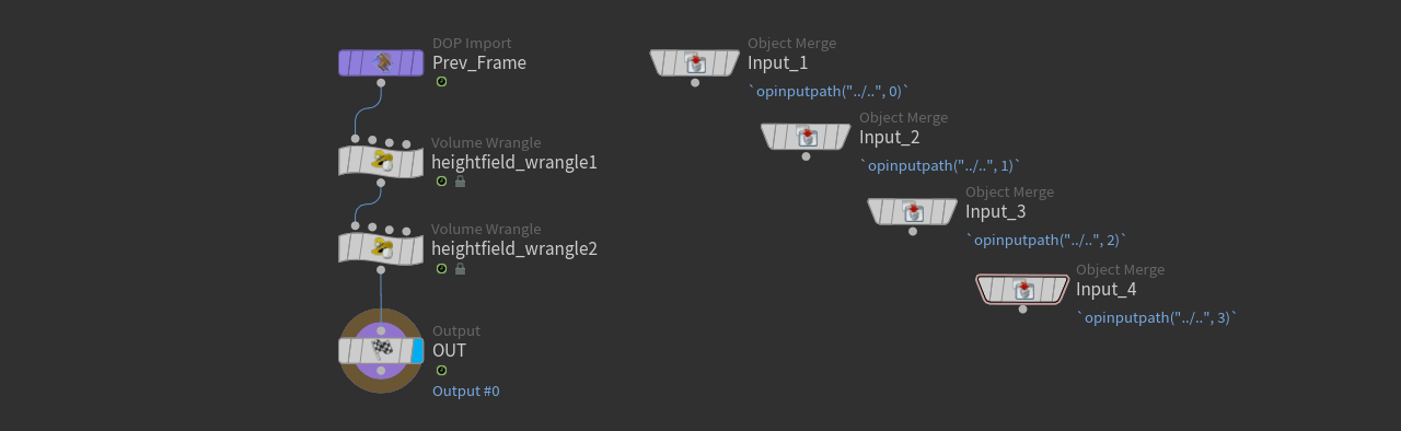
Put the Solver SOP between the copy and the clear nodes to connect its first input.
The node executes the simulation with a given number of Sub Steps. This number determines how often the wrangles will be applied to the terrain per frame. For the Abelian solver, a value around 5 gives good results. If you want the sand transport to become slower or faster, decrease or increase this value.
Then, double-click the solver to dive inside and add two HeightField Wrangle SOPs. The first inputs of the wrangle must be chained between the Prev_Frame and the OUT nodes. Now you have a working solver setup and it’s time to add the code.
Direction wrangle 
This wrangle contains the custom parameters for adjusting the solver. The script here also determines, in which direction the sand should move and writes this direction to the delta layer. The problem is that heightfield layer’s aren’t capable of storing vector values. Therefore, it’s necessary to represent the eight possible directions as numbers. Parameters that are required to control the sand transport will also be stored as detail attributes.
Use ⌃ Ctrl + C to copy the code below. With ⌃ Ctrl + V you can paste the script to the first wrangle’s VEXpression field.
// ============================================================================
// EROSION DIRECTION WRANGLE – Determines sand sliding direction based on slope,
// wind influence, and user-defined thresholds. This is the first step in the
// erosion-sedimentation cycle.
// ============================================================================

// --- Retrieve simulation parameters from the UI ---
float grid_resolution      = chf("grid_resolution");       // Size of each grid cell
float slope_threshold      = chf("slope_threshold");       // Minimum slope required for sand to slide
float scale_factor         = chf("scale_factor");          // Multiplier controlling erosion intensity
float sedimentation_scale  = chf("sedimentation_scale");   // Controls how much sediment accumulates in low areas
float wind_angle_deg       = chf("wind_direction");        // Wind direction in degrees (0° = +X, 90° = +Y)
float wind_bias_strength   = chf("wind_bias_strength");    // Strength of wind influence on sand movement

// --- Compute the effective slope threshold for sliding ---
float sliding_threshold = grid_resolution * slope_threshold;

/*
   Convert wind angle from degrees to radians and generate a unit vector
   pointing in the wind direction. This vector will be used to bias sand
   movement toward the wind.
*/
float wind_angle_rad = radians(wind_angle_deg);
vector base_wind_dir = set(cos(wind_angle_rad), sin(wind_angle_rad), 0);

/*
   Define the 8 possible neighbor directions:
   - 4 cardinal directions (left, right, up, down)
   - 4 diagonal directions (top-left, top-right, bottom-left, bottom-right)
   These are used to evaluate slope and determine possible sliding directions.
*/
vector dirs[] = array(
    set(-1,  0, 0), set( 1,  0, 0),
    set( 0, -1, 0), set( 0,  1, 0),
    set(-1, -1, 0), set( 1, -1, 0),
    set(-1,  1, 0), set( 1,  1, 0)
);

// --- Initialize array to store valid sliding directions ---
int slide_indices[];

// --- Cache current cell height and grid position ---
float h_self = @height;
int x = @ix;
int y = @iy;

/*
   Loop through all neighboring cells to evaluate slope.
   If the slope toward a neighbor exceeds the adjusted threshold,
   that direction is considered a valid candidate for sand sliding.
*/
for (int i = 0; i < len(dirs); i++) {
    vector dir = dirs[i];
    int nx = x + int(dir.x);
    int ny = y + int(dir.y);
    float h_neighbor = volumeindex(0, "height", set(nx, ny, 0));

    float slope = h_self - h_neighbor;
    float distance = length(dir); // 1.0 for cardinal, ~1.414 for diagonal
    float adjusted_threshold = sliding_threshold * distance;

    if (slope > adjusted_threshold) {
        append(slide_indices, i); // Store index of valid direction
    }
}

/*
   If there are valid sliding directions, choose one.
   The selection is biased toward the wind direction using a dot product.
   Directions aligned with the wind receive higher weights.
*/
int direction_code = -1;
if (len(slide_indices) > 0) {
    float weights[] = {};

    for (int i = 0; i < len(slide_indices); i++) {
        vector dir = dirs[slide_indices[i]];
        float bias = dot(normalize(dir), base_wind_dir); // Alignment with wind
        float weight = 1 + bias * wind_bias_strength;    // Wind bias scaling
        append(weights, weight);
    }

    /*
       Randomly select one direction from the weighted list.
       This introduces a stochastic approach while still favoring wind-aligned movement.
    */
    int pick = sample_discrete(weights, rand(@ix * 17 + @iy * 43 + @Time));
    direction_code = slide_indices[pick];
}

// --- Store the chosen direction as a float attribute for use in the next wrangle ---
@delta = float(direction_code);

/*
   On the first frame, store global parameters as detail attributes.
   These will be accessed in Wrangle 2 to ensure consistent values across voxels.
*/
if (@Frame == 1) {
    setdetailattrib(0, "sliding_threshold", sliding_threshold, "set");
    setdetailattrib(0, "scale_factor", scale_factor, "set");
    setdetailattrib(0, "sedimentation_scale", sedimentation_scale, "set");
}
Parameters 
The first script above contains definitions for six custom parameters. To add the parameters to the wrangle’s UI, click the ![]() Creates sparse parameter for each unique call of ch() button. Note that the values in the table below are just suggestions and it’s likely that you have to adjust them with your terrain.
Creates sparse parameter for each unique call of ch() button. Note that the values in the table below are just suggestions and it’s likely that you have to adjust them with your terrain.
| Parameter | Description | Value |
|---|---|---|
| Grid Resolution | This parameter makes the erosion structures resolution-independent. You should use the value from the HeightField SOP’s Grid Space parameter. |
n/a
|
| Slope Threshold |
Minimum slope required for sand to slide. Smaller values will consider less steep areas and you’ll get erosion in more areas. With very small values (<0.3), the results might look artificial.
|
0.7
|
| Scale Factor | With large height differences, you might see noise or other artifacts. Scale Factor parameter reduces this effect. You shouldn’t change the values unless you want to achieve a certain result. |
0.25
|
| Wind Direction | The solver uses a basic wind model to avoid noise patterns on the sediment structure. Here you can just the wind’s direction in degrees. Note that the impact of the wind model is limited. |
60
|
| Wind Bias Strength |
This parameter controls the maximum influence of the wind on a voxel. The combination of Wind Direction and high Wind Bias Strength (>50) can help to reduce the terracing effect.
|
1
|
| Sedimentation Scale |
With 0, you can turn off sedimentation completely. A value of 1 means mass-conservation and the amount of eroded sand equals the amount of sediment. Values greater than 1 will fill the terrain faster, values smaller than 1 will reduce the amount of sediment.
|
1
|
Erosion wrangle 
This script reads the encoded direction values of the delta layer to determine voxels with sliding sand. The script also updates the terrain’s height layer and applies the sedimentation process based on the custom parameters from the first wrangle.
Use ⌃ Ctrl + C to copy the code below. With ⌃ Ctrl + V you can paste the script to the second wrangle’s VEXpression field.
// ============================================================================
// EROSION APPLICATION & SEDIMENTATION WRANGLE – Applies sand movement based on
// previously computed directions, and adds sediment in low-lying regions.
// This is the second step in the erosion-sedimentation cycle.
// ============================================================================

// --- Retrieve global parameters stored in Wrangle W1 ---
float sliding_threshold     = detail(0, "sliding_threshold") * detail(0, "scale_factor");
float sedimentation_scale   = detail(0, "sedimentation_scale");

/*
   Define the 8 neighboring directions:
   - 4 cardinal directions (left, right, up, down)
   - 4 diagonal directions (top-left, top-right, bottom-left, bottom-right)
   These are used to evaluate incoming and outgoing sand flow.
*/
vector dirs[] = array(
    set(-1,  0, 0), set( 1,  0, 0),
    set( 0, -1, 0), set( 0,  1, 0),
    set(-1, -1, 0), set( 1, -1, 0),
    set(-1,  1, 0), set( 1,  1, 0)
);

// --- Cache current voxel position ---
int x = @ix;
int y = @iy;

// --- Initialize height change accumulator ---
float height_increment = 0;

// --- Retrieve own sliding direction from previous wrangle ---
int my_delta = int(@delta);
vector my_dir = my_delta >= 0 ? dirs[my_delta] : {0, 0, 0};

/*
   Loop through all neighbors to check if any of them are sliding sand
   toward this cell. If a neighbor's sliding direction points toward us,
   we receive sand from them.
*/
for (int i = 0; i < len(dirs); i++) {
    int nx = x + int(dirs[i].x);
    int ny = y + int(dirs[i].y);
    float neighbor_delta = volumeindex(0, "delta", set(nx, ny, 0));

    if (neighbor_delta >= 0) {
        vector neighbor_dir = dirs[int(neighbor_delta)];

        /*
           If the neighbor's direction is opposite to the current direction,
           it means sand is flowing into this cell.
        */
        if (length(neighbor_dir + dirs[i]) < 0.01) {
            height_increment += sliding_threshold;
        }
    }
}

/*
   If this cell is actively sliding sand away (i.e. has a valid direction),
   subtract sand from its height.
*/
if (my_delta != -1) {
    height_increment -= sliding_threshold;
}

/*
   If this cell is not sliding (i.e. stable), check if it lies in a depression.
   If the average height of its neighbors is higher, we simulate sedimentation
   by adding sand proportionally.
*/
if (@delta == -1) {
    float h_self = @height;
    float h_sum = 0;
    int count = 0;

    for (int i = 0; i < len(dirs); i++) {
        int nx = x + int(dirs[i].x);
        int ny = y + int(dirs[i].y);
        float h_neighbor = volumeindex(0, "height", set(nx, ny, 0));
        h_sum += h_neighbor;
        count++;
    }

    float h_avg = h_sum / count;
    float sediment_amount = clamp(h_avg - h_self, 0, sliding_threshold);

    // Add sediment scaled by user-defined factor
    height_increment += sediment_amount * sedimentation_scale;
}

// --- Apply accumulated height change ---
@height += height_increment;
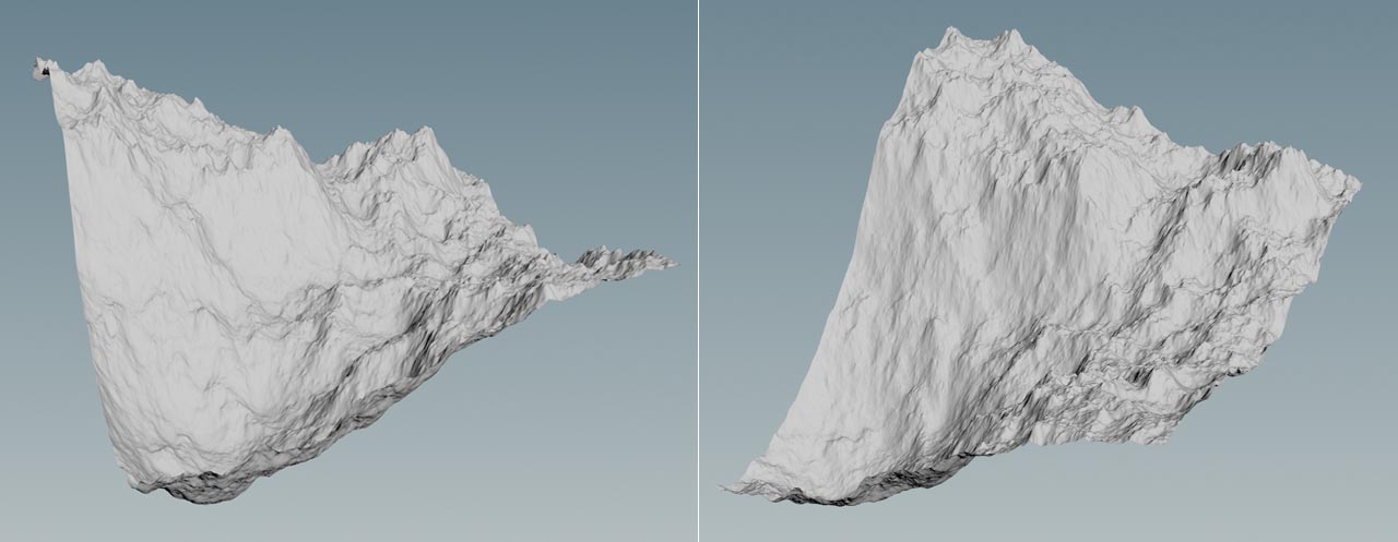
Result 
Once you've adjusted the parameters, you can go to the Playbar and click the ![]() Play button to start the simulation. The script should be rather fast and in most cases you won’t have to simulate for more than 50-70 frames.
Play button to start the simulation. The script should be rather fast and in most cases you won’t have to simulate for more than 50-70 frames.
The video shows how a terrain is transformed from rough and rocky mountains to an eroded landscape with debris mounds. To avoid a very smooth look, you can terminate the network with another HeightField Distort by Noise SOP with moderate settings to keep the sandy appearance.
When you look closely at the right part of the terrain, you can see how the sand is flowing down. To enhance this effect, the solver’s Sedimentation Scale was set to 1.6.