| On this page |
Overview 
SOP-based whitewater is an enhancement to the SOP FLIP fluids workflow. This system is scale-independent and lets you control the physical amount of whitewater without having to consider particle counts. You can work at low resolutions to find working settings, and reuse the values for a high-res pass. The SOP whitewater system supports the simultaneous creation of foam, spray, and bubbles.
Whitewater Lifecycle 
The solver takes care of birthing new whitewater particles, using the emission
volume created by the ![]() Whitewater Source node to
determine the amount. When Limit Emission is enabled, the present
distribution of whitewater particles is also considered, avoiding over-emission.
Whitewater Source node to
determine the amount. When Limit Emission is enabled, the present
distribution of whitewater particles is also considered, avoiding over-emission.
Aging and killing of particles is likewise handled by the solver. As simulation progresses, whitewater ages in an ordinary manner; however, particles do not have a prescribed lifetime. Instead, a death chance is dynamically calculated for each particle, taking into account its current condition. The following factors are considered when determining a particle’s dying probability:
-
age - Older particles are more likely to be killed.
-
depth - As depth varies, so does whitewater’s chance of dying, per values of the Aging Rates.
-
density - When erosion is enabled, whitewater density in a particle’s neighborhood is also used to augment its death chance.
Advanced users can further manipulate particle lives by accessing their
deathchance point attributes.
Note
Ignoring other factors, Lifespan is the statistical average for lifetime of whitewater particles.
Workflow 
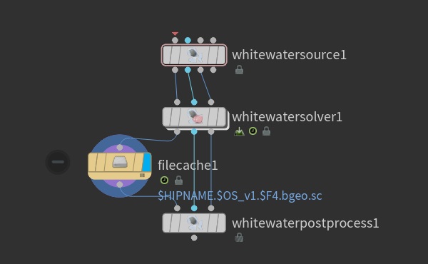
Pressing ⇥ Tab in the network editor and putting down a Whitewater Configure will generate and connect the 4 nodes for creating whitewater. This is a helpful starting point to see how the three whitewater nodes are wired together.
-
The
 Whitewater Source node generates the emission field for whitewater simulations.
 -
The
 Whitewater Solver sets and configures a Whitewater simulation inside a SOP network.
 -
The
Whitewater Post-process prepares the whitewater simulation for rendering. -
The
 File Cache node serves as a reminder that you should be caching your simulation before rendering.
Example 
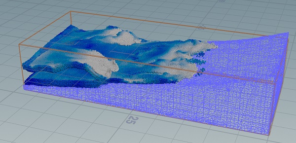
You can quickly generate a very simple whitewater simulation by pressing ⇥ Tab and putting down a FLIP Configure Beach Tank. This is a helpful example to look at when you first start, as it shows how FLIP Fluids are generated and how to apply whitewater to a FLIP simulation.
Whitewater sources 
There are several different ways to emit particles for whitewater. These options are available on the on the Sources tab of the ![]() Whitewater Source SOP.
Whitewater Source SOP.
Curvature
Uses the angle between the velocity of the particle and the surface normal to calculate emission. If an angle is lower than the value of Max Velocity Angle, whitewater will be emitted. This ensures that whitewater is only created on the leading edges of waves.
Acceleration
Calculates emission based on changes in the fluid’s velocity. It detects the areas where particles are rejoining the existing parts of the fluid, such as when a wave that is about to crash starts falling.
Vorticity
Looks at the magnitude of rotation inside a velocity volume to identify churning areas of the fluid, which generally occur deeper below the surface. For example, when a wave crashes.
Pressure
Emits particles based on the alignment between the pressure and surface gradients. If the two vectors are pointing in opposite directions, you will have calm static water and nothing will be emitted. However, as soon as you have a wave crashing, the pressure gradient will be pointing in the same direction and particles will be emitted.
Splash
Acts directly on the points and uses relative density. High density refers to particles that are densely packed and close to neighboring particles, whereas low density is when particles are more isolated from their neighbors. In this example, particles are emitted in areas that have low relative density and not emitted where particles are densely packed.
Deformation sources 
Another method of sourcing whitewater is deformation based emission. This method identifies stretching, squishing, and scaling of the fluid surface. Stretch corresponds to the expansion of the surface along a specific direction. Squish corresponds to the compression of the surface along a specific direction. Surface scale corresponds to how much the surface compresses (negative values) or expands (positive values) considering all directions. These options are found on the Deformation sources tab of the ![]() Whitewater Source SOP.
Whitewater Source SOP.
Squish
Emits particles in areas of the surface that are compressed. For example, you can see a small ripple where the surface is pinching.
Stretch
Emits particles in areas of the surface that are extending.
Scale
Emits particles based on how much the surface compresses or expands in all directions.
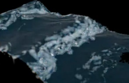
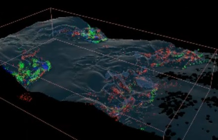
Visualizing whitewater 
The Visualization tab on the ![]() Whitewater Source node lets you turn on visualization for all of the different emission types that are activated. The following example shows visualizations of the Curvature (red), Acceleration (green) and Deformation (blue). The displayed color is chosen based on the most dominant criteria. So in this example, areas that are green mean that acceleration based emission is dominant over curvature and deformation. This doesn’t mean that emission wouldn’t be activated by another criteria. It just displays the most dominant one at that frame.
Whitewater Source node lets you turn on visualization for all of the different emission types that are activated. The following example shows visualizations of the Curvature (red), Acceleration (green) and Deformation (blue). The displayed color is chosen based on the most dominant criteria. So in this example, areas that are green mean that acceleration based emission is dominant over curvature and deformation. This doesn’t mean that emission wouldn’t be activated by another criteria. It just displays the most dominant one at that frame.
Tips 
-
By default,
emit,surface, andvelare all output through the first output of the node. However, you can choose to only output the emission field to cache it in isolation and save some disk space. To enable this option, turn off the Output Fluid Fields checkbox on the Fluid Fields tab. -
You can turn on the Extra Sources feature by connecting geometry to the fourth input. This is where you can connect another way of sourcing whitewater and it will convert those points into emission volume for the simulation.
-
If you don’t see enough whitewater or if you see too much whitewater, you could try adjusting the sourcing. However, most of the time the better approach is to revisit the FLIP simulation, because the momentum and energy comes from the underlying simulation and is transferred to the secondary simulation.
-
If the default ranges are not adequate for your specific scene, you can click the Compute Range From Data buttons beside the various sources to give you a better starting point. These values will still have to be refined, but should provide a better estimate of suitable Min and Max values.
-
To preview the generated particles, turn on visualizations in the Visualization tab and use the fourth output. This will show visualization of the source types.
-
You can also export raw attributes on the points by turning on the Output Emission Attributes checkbox. These are the raw attributes coming from the FLIP simulation.
-
All sources on the Sources and Deformation Sources tabs are affected by the Masks tab. It does not affect Extra Sources.
Whitewater solver 
There are several ways to control the amount of whitewater in a simulation. The following are some of the most common ways.
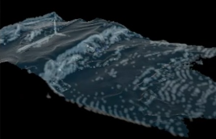
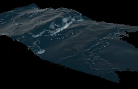
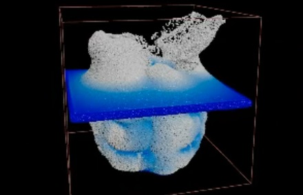
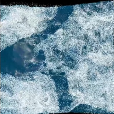
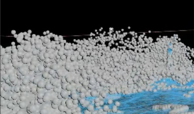
The Whitewater Scale parameter on the Setup tab of the ![]() Whitewater Solver SOP controls the separation between nearby whitewater particles. Reducing this parameter increases the number of particles in the simulation (with cubic scaling). For example, a value of
Whitewater Solver SOP controls the separation between nearby whitewater particles. Reducing this parameter increases the number of particles in the simulation (with cubic scaling). For example, a value of 0.1*2 will result in the amount of particle being divided by 8. The first image shows 600,000 particles before applying Whitewater Scale, and the second images shows 75,000 particles after.
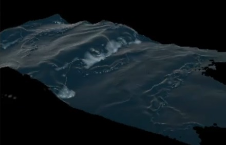
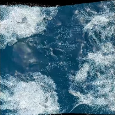
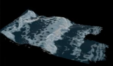
Another way to control the amount of whitewater is by using the Emission Amount parameter on the Emission tab of the ![]() Whitewater Solver SOP. This parameter is a simple multiplier for the amount of emitted whitewater (scales linearly). So if you want to half the amount of emitted particles you use a value of
Whitewater Solver SOP. This parameter is a simple multiplier for the amount of emitted whitewater (scales linearly). So if you want to half the amount of emitted particles you use a value of 0.5. The first images shows 600,000 particles before applying a 0,5 reduction of particles, and the second images shows 300,000 particles after.
Wind 
Wind only affects spray particles in whitewater. When particles are lifted off the surface, they are carried by the wind that is defined on the Forces tab of the ![]() Whitewater Solver SOP. There are also Wind Shadow options, to make the spray behave more realistically. The Enable Collider Shadow checkbox lets you use collision geometry to block wind from affecting the spray. In this case, the wind is being occluded by the collider and the particles simply obey gravity. There is also an option to Enable Water Shadow, which uses the water surface (such as a wave) to block wind from affecting the spray behind it.
Whitewater Solver SOP. There are also Wind Shadow options, to make the spray behave more realistically. The Enable Collider Shadow checkbox lets you use collision geometry to block wind from affecting the spray. In this case, the wind is being occluded by the collider and the particles simply obey gravity. There is also an option to Enable Water Shadow, which uses the water surface (such as a wave) to block wind from affecting the spray behind it.
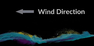
In this example, the spray is yellow, the foam is blue, and the bubbles are purple. When the particles go behind the wave, they stop being carried by the wind and fall linearly back to the surface.
For information on other forces, see the DOP Whitewater help page.
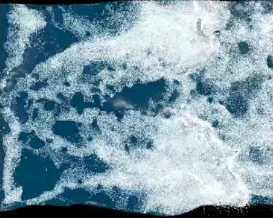
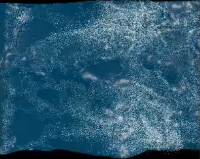
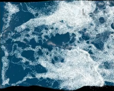
Foam erosion 
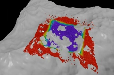
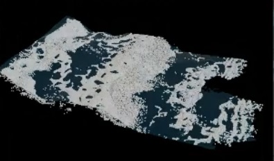
You can Enable Erosion of foam on the Foam tab of the ![]() Whitewater Solver SOP. This preserves foam in denser areas and erodes it in sparser regions. The parameters in this section allow you to set how fast the foam disappears and the density at which whitewater is protected from erosion. The following image shows the before and after of Erosion Strength at
Whitewater Solver SOP. This preserves foam in denser areas and erodes it in sparser regions. The parameters in this section allow you to set how fast the foam disappears and the density at which whitewater is protected from erosion. The following image shows the before and after of Erosion Strength at 0.5*100 and Preservation Strength at 0.5*0.
This feature is useful in simulations where a lot of whitewater is being emitted and starts to look like a big white patch with no details. Adding erosion can be used to get more of the particles to disappear faster and create more holes where you can see the surface of the water.
Tip
Turning on the Relative Density mode on the Visualization tab can be useful when working with erosion settings.
Repellants 
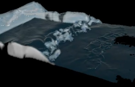
You can Enable Repellants to create and maintain repellant particles that push whitewater away and result in an organic cellular foam structure. These controls are located on the Foam tab of the ![]() Whitewater Solver SOP. The repellants are represented by red dots in the following image.
Whitewater Solver SOP. The repellants are represented by red dots in the following image.
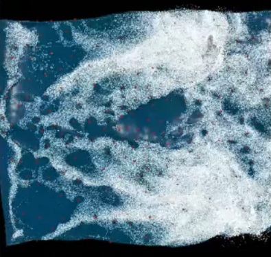
There is a lot of variation in the radius of repellants and noise applied to make the simulation look as organic as possible. This helps create interesting cellular patterns in the whitewater. Note that the red dots are simply a visualization used for this example to show the center of the repellant to more easily illustrate the different sizes and noise patterns.
For more information on repellants, see the DOP Whitewater help page.
Tips 
| To... | Do this |
|---|---|
|
Make the foam patches disappear faster |
Increase the Erosion Strength parameter on the foam tab. |
|
Prevent particles from being projected to the surface very quickly |
The default settings in the Adhesion section on the Foam tab are for large scale simulations. Tweaking these parameters, including lowing the Stiffness by Depth ramp, will solve this issue resulting in particles floating to the surface more naturally. |
|
Visualize attributes like relative density |
You can use the Mode dropdown menu on the Visualization tab to visualize attributes such as Depth, Speed, State, and Relative Density. |
Whitewater postprocess 
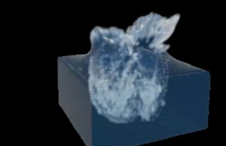
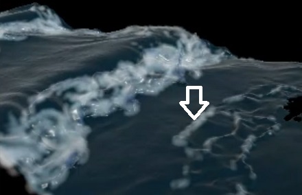
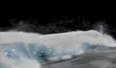
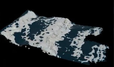
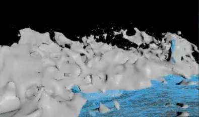
The ![]() Whitewater Post Process SOP prepares the whitewater simulation for rendering. This is where you can choose to output your whitewater as modified Particles, a Fog Volume along with a velocity field, or a Mesh representation of the whitewater simulation, which can be rendered as a uniform volume.
Whitewater Post Process SOP prepares the whitewater simulation for rendering. This is where you can choose to output your whitewater as modified Particles, a Fog Volume along with a velocity field, or a Mesh representation of the whitewater simulation, which can be rendered as a uniform volume.
Particles
The default output for whitewater. It outputs a modified particle representation of the whitewater simulation. This option is useful when you want lots of fine splashy details. For example, if you're simulating a wave crashing on a rock.
Fog Volume
Outputs a volume representation of the whitewater simulation with a velocity field. This option is useful when you want to see the light travel through and be absorbed by the whitewater.
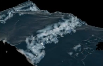
Mesh
Outputs a mesh representation of the whitewater simulation with transferred velocity. This option is useful when you want very defined sharp edges between areas with foam and no foam.
Tips 
-
You can use the Flatten Outside Bounding Box options on the Domain tab of the
Whitewater Post Process SOP to flatten the whitewater particles to the water level offset by their depth attribute. This is useful when you have a fluid simulation that you want to blend with a procedural ocean simulation. Turning this on will prevent the whitewater from looking like it’s floating above the surface of the other particle fluid.