The ocean spectrum creates a velocity field that moves the particles. The parameters are just suggestions to give you an idea of how create waves. Of course, you can experiment with different settings.

1. Add an Ocean Spectrum SOP node and open its parameters.

2. Set Resolution Exponent to 8 to get enough detail and catch smaller waves. You can consider this parameter as the spectrum’s quality level.

3. The ocean spectrum’s scale is controlled through Grid Size. If the value is smaller than the domain’s XZ size, the spectrum will be tiled and you might see repetitions or a scale mismatch. Here, enter a value of 35 to cover the domain’s entire XZ plane.

Add an Ocean Evaluate SOP node and connect its second input with the Ocean Spectrum’s output. Although the Ocean Evaluate node’s first input is tagged as required, it’s not mandatory here to add a deforming geometry. Finally, connect the Ocean Evaluate node’s output to the FLIP Solver’s fourth input (Boundary Flow). This connection transfers the waves' velocities and pressure to the FLIP fluid particles.

The FLIP Container SOP node defines the simulation domain’s dimensions and resolution. Make the domain large enough, for example 20 m by 20 m in the XZ plane. Also make the domain high enough to catch bigger waves. A value of 10 m is a good start. Instead of changing the Domain ▸ Size parameters, you can also connect a Box SOP node to the container’s input. It might be easier for you to control the domain’s dimensions through a geometry node.

Particle Separation determines the fluid’s resolution and finally the number of particles. The smaller the value, the more voxels and the more particles you’ll finally get. More voxels and particles also mean longer simulation times and higher memory consumption. In return you will get more details and smaller waves. Considering the domain’s size, a value between 0.2 and 0.1 is good for previews to save simulation time. For the final version, use 0.05.

1. Add a FLIP Solver SOP.

2. Connect the container’s three outputs to the solver’s first three inputs.

3. Connect the Ocean Evaluate node’s output with the 4th input of the FLIP Solver node.

4. Go to the Boundary Behavior section. The most important choice is, which Type you want to use: Velocity Driven or Pressure Driven. In this scene, there is no “right” or “wrong”, and the Type is mainly a matter of preferences. Scenes with Pressure Driven tend to be more turbulent and splashy.

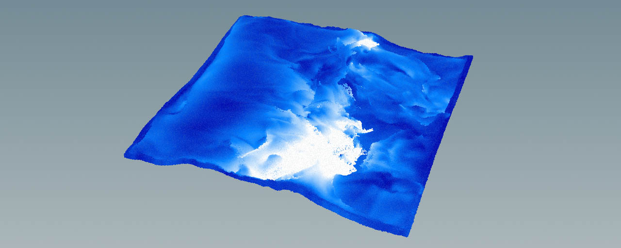
When you turn on the node’s blue Display/Render flag, Houdini creates the water surface, based on the spectrum waves. You’ll also recognize a particle band around the domain’s outside. This is the area where new particles are sourced. Particles, hitting the domain’s inside, are deleted. This in-and-out flow creates an equilibrium and keeps the number of particles almost constant throughout the simulation (unless you add particles from another source).

You can simulate the fluid and cache the results to the computer’s memory. The FLIP Solver has a default cache limit of 5,000 MB, which is normally not enough for a long or complex simulation. The result will also be lost when you close the project. If you have enough RAM and don’t want to store the simulation in the computer’s memory, do this:

• Open the FLIP Solver’s Simulation tab and increase Cache Memory (MB).

A better solution is to save the simulation to disk:

1. Add a File Cache SOP node after the solver.

2. Connect the input with the solver’s first output.

3. If you keep the entry under Base Folder, you can find the cache files in the project directory ($HIP) under geo.

4. Click Save to Disk (locks the UI) or Save to Disk in Background (the UI remains responsive).

5. Load from Disk is turned on automatically and you can scrub the timeline to see the result in the viewport.

You can observe waves moving and breaking. Waves also vanish at the domain’s borders, while new particles are sourced from the source band around the domain. The video below shows a simulation with Type set to Pressure Driven.

In this clip, Type is Velocity Driven. The waves are less splashy and the ocean surface is calmer.