In this example, the scene contains a water tank and a rock formation. The low-resolution guided ocean segment is created from an ocean spectrum. Start with the domain.

1. Create a Box SOP and set its Size to 30,7,15.

2. Add a FLIP Container SOP node, and connect it with the output of the box.

3. Add a rock object. You can use imported geometry or a Houdini model. To remove particles inside the object, the model has to be closed and should intersect the container’s lower base.

4. If necessary, scale and rotate the rock object.

5. Add a FLIP Collide SOP node and connect the first three inputs with the outputs of the FLIP Container node.

6. Connect the rock object with the FLIP Collide node’s 4th input.

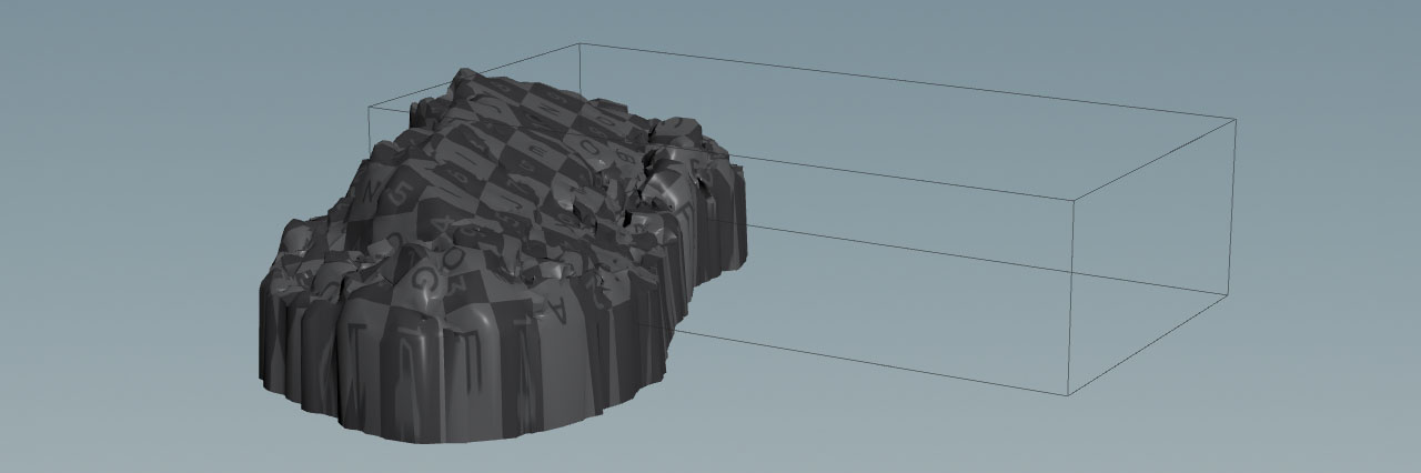
The image shows the the domain’s outlines with the rock, intersecting the lower base.

The fluid surface is created through an ocean spectrum, connected to the solver. Velocity and pressure information is transferred to the FLIP particles and drive the simulation.

1. Start with an Ocean Evaluate SOP node.

2. In the Geometry tab, turn on Preview Grid to see the effect of your changes.

3. Open the Volumes tab.

4. Turn on Surface SDF.

5. Turn on Velocity and Hyrodstatic Pressure. The latter option is only relevant with the solver’s default pressure boundary. Pressure-driven simulations tend to be more turbulent.

6. For Size you can use the domain’s dimensions (here: 30,7,15). Add 5 units to each value to be on the safe side (35,12,20).

7. From the Uniform Sampling dropdown menu, choose By Size.

8. Set Div Size to 0.15.

The Ocean Spectrum SOP is responsible for the ocean’s overall dynamics and the height of the waves.

1. Add an Ocean Spectrum node.

2. Connect the output with the 2nd input of the Ocean Evaluate node.

3. Change Resolution Exponent to 8 to get more surface details.

4. Open the Wind tab.

5. Change Spectrum Type to Philips.

6. Depending on where the rock is positioned, adjust Direction to make the waves move towards the rock. In this scene, the value is 180 (negative X direction).

7. Set Speed to 6 to get a wavy and turbulent surface.

8. Change Directional Bias to 6 to make more waves moving along the adjusted Direction.

9. Open the Amplitude tab and set Scale to 2. You can increase or decrease this value if the waves' height doesn’t match.

The FLIP Solver SOP is the setup’s core element and performs the actual simulation.

1. Add a FLIP Solver node.

2. Connect the first three inputs with the outputs of the FLIP Collide node.

3. Connect the fourth input with the output of the Ocean Evaluate node.

4. Go to the FLIP Container and right-click Particle Separation. From the menu, choose Copy Parameter.

5. In the Setup tab, go to General ▸ Particle Separation and turn it on.

6. Right-click the value, and choose Paste Relative Reference. Now, both parameters are connected. When you change the container’s value, the solver’s value is automatically updated.

Below you can see the result of the low-resolution simulation with approx. 350,000 particles.

The idea is to define a region of interest near the rocks and create a high-resolution close-up from the existing base simulation.

1. Create another Box SOP node.

2. Find an interesting region where you want to see more details. Scale the box and move it to this region.

3. Add a second FLIP Container node and set Particle Separation to 0.025.

4. Connect the box with the container’s input.

The high-resolution version requires its own FLIP Collide node. You can use the default settings.

1. Add a FLIP Collide node.

2. Connect the first three inputs with the container’s outputs.

3. Connect the rock object with the collide node’s 4th input.

A second solver simulates the high-resolution version within the specified segment. This new solver uses the information from the first solver by connecting both nodes.

1. Add a FLIP Solver node.

2. Connect its first three inputs with the outputs of the FLIP Collide node.

3. Connect the 4th input of the new solver with the first output of the existing low-resolution solver.

4. Select the high-resolution container and right-click Particle Separation. From the menu, choose Copy Parameter.

5. Go to the high-resolution solver’s Setup sub-pane.

6. Turn on Particle Separation.

7. Right-click Particle Separation and choose Paste Relative References to establish a connection between both parameters.

Here is the result of the high-resolution ocean segment: