1. ⌃ Ctrl-click the Sphere tool from the Create shelf tab to create a sphere at the origin.

2. With the sphere selected, go to the Rigid bodies shelf tab and click the RBD Hero Object.

3. Click Play on the playbar at the bottom of the Houdini window.

The sphere falls because it’s now a simulated object. When you first create a simulated object, Houdini automatically creates a simulation network at the obj level so it has somewhere to put the nodes defining the simulated object’s behavior. The network appears in the network editor at the obj level as a node called AutoDopNetwork.

If you double-click AutoDopNetwork to go inside, you can see the network Houdini created to define the simulation. You may want to press L to have Houdini lay out and rearrange the network.

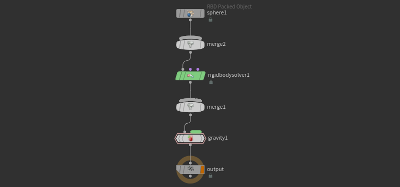
The network is quite simple, but all by itself demonstrates several basic concepts of Houdini dynamics, starting with the fact that it consists of an object, a solver, and a force.

A dynamics object holds the parameters necessary to describe some thing being simulated. In the network above, the sphere object’s node has parameters for where to get the simulated object’s geometry (it references the sphere object you created), the density, temperature, friction of the object, its initial position, rotation, velocity, and so on.

A solver does the work of calculating how simulated objects behave. They look at the state of the simulation and use their internal rules to modify it at each time step. In the network above, the RBD solver simulates the motion and collisions of the rigid body sphere.

A force is a piece of information you can attach to objects (all objects in the scene, or individual objects) that says, for example, “this object is affected by a wind” or “this object’s motion is slowed by drag”. In the network above, the Gravity node attaches “force data” to any objects above it (the sphere). When the solver sees the force data on the object, it knows to pull the sphere downward at each time step to simulate the effect of gravity. Tools on the Drive Simulation shelf tab let you add forces to a simulation.

These are the main solver types

• Rigid bodies

• Fire and smoke

• FLIP fluids

• Oceans and ripples

• Vellum fluids and grains

• Vellum cloth, ropes and softbodies

• Particle systems

• Finite elements

In other network types, Merge nodes combine the output of the nodes that feed into them. In dynamics networks, Merge nodes create relationships. Relationships are a special type of data that describe which objects affect which other objects.

The main type of relationship in dynamics is a collision relationship, meaning objects will change their shape/motion/behavior when they collide with other objects. There are also constraint relationships (such as pins and springs) in RBD, wire, and cloth simulations.

The important thing to remember about relationships is that they take time to calculate, so to optimize the simulation, you should only create relationships between objects that really need to interact, and you should look for ways to use one-way relationships (where one object affects another but not the other way around).

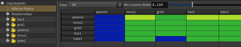
The Geometry Spreadsheet contains an affector matrix for visualizing which objects affect which. To access the affector matrix, click the project’s Dop Network OBJ and open the Geometry Spreadsheet tab. Note that the project must contain the RBD objects you want to inspect. In the spreadsheet’s hierarchy tree on the left there is an Affector Matrix branch. Click it to see the the objects' relations.

See visualizing dynamics.

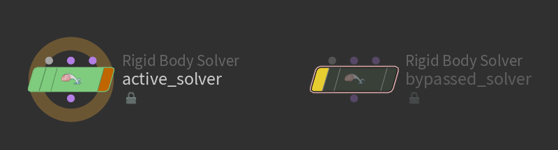
The orange flag marks the “output” or “endpoint” node of the network: only nodes above and including the node with the Output flag will be part of the simulation. There can only be one node with an active Output flag per network.

DOPs also have a Bypass flag so you can check the state of the simulation with and without a given node, usually for debugging the creation of data in the Geometry Spreadsheet (see below).

If you want to animate the presence of objects or data, keyframe the given node’s Activation parameter. When Activation is non-zero, the node is active and affects the network. When Activation is zero, the node has no effect, similar to having the bypass flag on.

The Geometry Spreadsheet is your window into the underlying objects and data of a simulation. You can create a new Geometry Spreadsheet pane in a tab. The tree on the left side represents the objects in the scene and categories such as relationships, with branches representing the hierarchy of data attached to each object. The right side shows the fields of the data piece selected on the left side and their values.

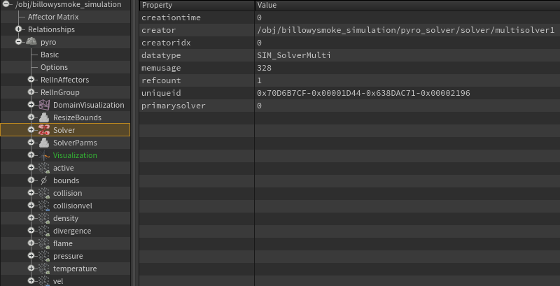
This pane is very useful for examining the structure of the simulation. You can see which data is attached to which at the current frame and with the current output node, names and unique ids of data packets, as well as the values that make up the data.

The Geometry Spreadsheet updates dynamically as you play the simulation. This is very useful when you want to see how data changes over time, but it slows down playback of the simulation. You can use the arrows on the pane divisions to “collapse” the Geometry Spreadsheet when you don’t need it to make simulation playback smoother.

Network evaluates top down, left to right. For a node with multiple inputs, it evaluates top to bottom on its first input, then top to bottom on its second input, etc.

To make a solver’s collision detection more accurate, increase the solver’s Maximum substeps parameter. This will usually make the simulation take longer to calculate.

You can also increase the resolution of the simulation globally with the Timestep parameter on the DOP Network node containing the simulation. You can also change sub-stepping directly on the solver object.

The dynamics engine calculates the simulation in time steps: the amount of time between the points where Houdini stops and re-calculates the state of the simulation. Normally this is some multiple of the frame time (the length of time Houdini displays each frame, e.g. 1/24th of a second at 24 FPS), but that’s not necessary. Long time steps makes it easier for Houdini to run the simulation, but give less accurate results. Smaller time steps take longer to calculate, but give more accurate results.

To set the time step for a dynamics network, open the parameters for the DOP Network object, click the Simulation tab, and set the Time step parameter.

In individual solver nodes in a dynamics network, you can control the number of sub-steps the solver breaks the default time step into. This lets you increase the simulation’s granularity for just one solver, without increasing it for every calculation in the entire simulation by changing the time step.

To control sub-steps in a solver, set the solver’s Minimum substeps and Maximum substeps parameters. Increase the Minimum substeps value to have the solver break each time step into more solving steps. It’s helpful to limit the Maximum substeps to make sure the simulation eventually finishes in a reasonable amount of time.

In the dynamics set-up, Houdini created when you turned the sphere into a simulated rigid body object, the dynamics network imports the sphere’s geometry (in the RBD Object DOP node at the top of the dynamics network) out of the geometry network, and simulates its motion.

Then the original sphere Geometry object’s network imports the motion from the simulation back into the object (in the DOP Import SOP node at the bottom of the geometry network).

So what you render is the original object, after it has its geometry, position, etc. modified by the dynamics network. The AutoDopNetwork object has its blue display flag (the button on the right side of the node) off by default, meaning it won’t render.

This is simply because Mantra is really set up to render objects, so importing the simulation motion back into an object gives you all the controls for rendering that objects have. And while technically you can render a dynamics network at the object level directly, its geometry will usually include a lot of guides and user interface geometry you probably don’t want to render.

Since solvers are simulating real-world physical processes, they need a way to relate numbers in the scene to real-world units. The designers of Houdini’s dynamics system decided to simply use the base SI units: 1 Houdini unit is equal to 1 meter, weights are always specified in kg, and times are always specified in seconds. Other units are always derived from meters, kilograms, and seconds (for example, density is specified as kg/m³).