Simulations consist of objects and data. Objects are merely repositories of data. When you see an object, such as an RBD ball, in your scene, it’s because the object has Geometry data attached to it, which by convention Houdini draws in the viewer and renders.

The data attached to objects is, in some sense, arbitrary: it can be pretty much anything. There are no constraints on how a piece of data is named or what it contains. But only certain names and types of data are meaningful to solvers.

Solvers do the work of calculating how simulated objects (RBD objects, wires, cloth surfaces, fluids, etc.) behave. They look at the data attached to objects (and may attach some of their own) and use it to run the simulation.

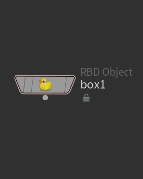
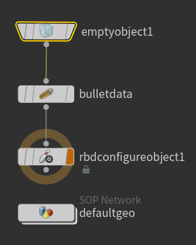
When you create a simulation object from the shelf, Houdini creates a high-level object, such as an RBD object. You can dive into the RBD object node to see that it’s really an Empty object with the right data attached - the data the RBD solver needs to simulate the object.

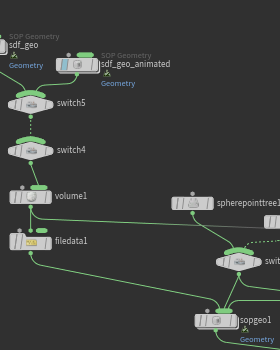
High level RBD object.	Inside is an empty object with an RBD configure object node.	Inside the RBD Configure DOP object node is a bunch of data attachments.

(Many dynamics nodes are implemented this way, as digital assets, where high-level nodes encapsulate networks that in the end are just attaching data to objects for the solvers to interpret.)

Solvers will use data it knows about and ignore other data. So, you can attach data useful to another solver (such as scalar data), or any arbitrarily named data, to an RBD object and the RBD solver will happily ignore it.

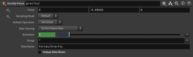
Solvers do the work of calculating how simulated objects (RBD objects, wires, cloth surfaces, fluids, etc.) behave. They look at the data attached to objects (and may attach some of their own) and use it to run the simulation. For example, the RBD solver will look at the physical data, such as density, and forces, such as gravity, attached to an object to determine where to move it (updating its position data). If an object doesn’t have a solver attached to it, it won’t do anything when the simulation runs.

(OK, that’s not exactly true… if you really wanted to, you could use expressions in the data fields that are meaningful to the viewer, such as Position, to make simulated objects move without a solver. But it wouldn’t be nearly as much fun!)

The solver that should control an object is attached as another piece of data on the object. Different types of simulated objects can affect each other (for example, RBD objects displacing smoke). Objects cannot be controlled by multiple solvers, but you can attach a solver that itself uses multiple solvers, such as a Blend Solver DOP. See below for more information on combining solvers.

Houdini cooks dynamics simulations in a two step process:

1. Process the network to establish objects and data attachments.

2. Run solvers on the processed data tree.

For more information see DOPs input and output.

See caching simulated geometry to disk.

In a dynamics node that attaches data, each field has a pop-up menu that controls when the values on the right side are set on the input objects.

The default is Set initial, which sets/imports the data at the first frame of the simulation.

If you are importing values or geometry from outside DOPs where what is being imported changes (or may change) depending on the frame (for example deforming geometry or values referenced from other networks that use a time-dependent expression), you should change the menu for any parameters that need the updated value to “Set always”.

Set always is quite a bit slower, since it must constantly rewrite the data tree, so you shouldn’t turn it on unless you really need it, and turn it on for as few parameters as possible.

Houdini sorts out the objects in the scene based on relationships to determine the order in which to solve them. For one-way relationships, affectors are solved before the affected objects. Wherever a mutual relationship exists, or wherever a hierarchical group of relationships creates a loop, all relationships in that group must be solved simultaneously.

Simultaneous solving is really pseudo-simultaneous, because computers are sequential and can’t work with truly simultaneous events, so Houdini tries to work out a close approximation through an iterative process:

1. Apply forces to objects in the order - left to right, top to bottom (in the network).

2. Look for collisions.

3. If anything collided, feed the collision forces back into the objects. For static objects this feedback step is optimized out.

4. Repeat until no collisions or Max feedback loops is reached.

   The Max feedback loops parameter on the DOP Network containing the simulation limits the number of collision feedback loops Houdini will run, to speed up the simulation and prevent infinite loops.

The best order for solving RBD simulations is to evaluate the heavy objects first, before the light objects. When wiring nodes manually, you can try to wire heavy objects to the left of light objects in Merge DOP nodes. When creating networks automatically, Houdini will assume that particles (solved by the particle solver) are light, and try to wire them to the right of other objects. If you're simulating heavy particles, you may want to change the wiring order.

Houdini includes several utility solvers for setting up more advanced networks.

• Multiple Solver DOP runs multiple solvers in order on the same objects.

• Blend Solver runs multiple solvers and blends between their effects, based on blend factor data on each object. Use the Blend Factor DOP to attach blend factor data to each object.

• Switch Solver DOP routes objects to different solvers based on a piece of switch data on each object. Use the Switch Value DOP to attach switch data to each object.

  The switch solver is similar to the Switch DOP node, but where the Switch node operates during the data attachment step (and so can affect which data gets attached to which objects), the Switch Solver runs in the solve step (and so can see all data attached to all objects).

• Script Solver DOP runs a script that can potentially change data, update positions, etc. Several HScript commands, expression functions, and HOM classes exist to enable writing scripts to modify dynamics simulations.

• Copy Data Solver DOP