| On this page | |
| Since | 16.0 |
The Cloth Object DOP creates a Cloth Object inside the DOP simulation. It creates a new object and attaches the subdata required for it to be a properly conforming Cloth Object. Cloth objects can be simulated using the FEM Solver.
You can use any polygonal geometry in SOPs to create your cloth object. Your cloth geometry should satisfy guidelines that ensure a fast-running and good looking simulation.
See cloth forces and cloth collisions for more information.
Using Cloth Object 
-
Select the object to make into a cloth object.
-
Click the
 Cloth Object tool from the Cloth tab.
Parameters 
Model 
Stiffness Multiplier
This is a multiplier for all the internal stiffnesses of this object.
Damping Ratio
This controls how quickly the object stops deforming.
Mass Density
This is the amount of mass per volume.
Thickness
This determines the volume of the cloth per area.
Stretch Stiffness
This determines how strongly the object resists local stretching in the U and V directions (see the materialuv attribute).
Shear Stiffness
This determines how strongly the object resists local shearing between the U and V directions (see the materialuv attribute).
Bend Model
This determines the type of model that’s used for internal forces that resist bending.
Weak Bend Stiffness
This determines how strongly the object resist local bending under the weak bend model
Strong Bend Stiffness
This determines how strongly the object resist local bending under the strong bend model.
Seam Angle
This prescribes the rest angle between different panels.
Friction
This controls the strength of friction forces at contacts
Deformation 
Initial 
Initial State
The path to the SOP node with the initial connectivity, position and velocity.
Rest 
Rest Shape
The path to the SOP node that defines the rest shape.
Target 
Target Deformation
The path to the SOP node with target deformation.
Target Strength
Strength density of the distributed soft-constraint force field that tries to match the target position.
Target Damping
Damping density of the distributed soft-constraint force field that tries to match the target velocity.
Import Target Geometry
This option allows you to specify and animate the target positions that are used by the simulation inside the SOP network (without having to use a SOP solver). The option defines whether the target positions should be imported from a SOP geometry node at each frame. When enabled, the solver will copy target positions from the point attribute targetP of the SOP geometry node onto the attribute targetP on the simulation geometry at each frame. If no targetP exists, then the P attribute from the SOP geometry node is copied instead.
Target Geometry Path
The path to the SOP node that will serve as the source of the target positions. The positions should be stored in an attribute with the name targetP. If this attribute is not found, the P attribute is used as a fallback.
Stiffness
This coefficient determines how strongly the finite element solver tries to make the point positions match the target point positions. The solver creates an imaginary potential force for this purpose.
Damping
This coefficient determines how strongly the finite element solver tries to make the point velocities match the target point velocities. The solver creates an imaginary dissipation force for this purpose.
Collisions 
Collide with objects
If enabled, the geometry in this object will collide with all other objects. These other objects may belong to the same solver or they may be be ![]() Static Objects,
Static Objects, ![]() RBD Objects, or the
RBD Objects, or the ![]() Ground Plane. When the Collision Detection parameter on the Static Object is set to Use Volume Collisions, then the polygon vertices will be tested for collision against the signed distance field (SDF) of the Static Object. When Collision Detection is set to Use Surface Collisions, then geometry-based continuous collision detection is used. The geometry-based collisions collide points against polygons, and edges against edges.
Ground Plane. When the Collision Detection parameter on the Static Object is set to Use Volume Collisions, then the polygon vertices will be tested for collision against the signed distance field (SDF) of the Static Object. When Collision Detection is set to Use Surface Collisions, then geometry-based continuous collision detection is used. The geometry-based collisions collide points against polygons, and edges against edges.
When geometry-based collisions are used, only polygons and tetrahedrons in the ![]() Static Object are considered. Other types of primitives, for example spheres, are be ignored. The geometry of the external objects (e.g. Static Object) is treated as being one-sided; only the outsides of the polygons, determined by the winding order, oppose collisions.
Static Object are considered. Other types of primitives, for example spheres, are be ignored. The geometry of the external objects (e.g. Static Object) is treated as being one-sided; only the outsides of the polygons, determined by the winding order, oppose collisions.
When volume-based collisions are enabled, only points will be colliding against the volumes, not the interiors of polygons and tetrahedrons. When colliding against small volumes, this may mean that you need to increase the number of points on your mesh to get accurate collision results.
Collide with objects in this solver
When enabled, this object will collide with other objects that have the same solver. These collisions are handled using continuous collision detection, based on the geometry (polygons and/or tetrahedrons). For collisions between objects on the same solver, the polygons are treated as two-sided. Both sides of the polygons collide. The surface of a tetrahedral mesh only collides on one side: the outside.
Collide within this object
If disabled, then no two polygons within this object can collide with each other.
Collide within each component
If disabled, then no two polygons that belong on the same connected component may collide with each other.
Collide within each fracture part
This option only has an effect when fracturing is enabled on the solver. If disabled, then no two polygons that belong on the same fracture part may collide with each other. Fracture parts are controlled by the integer-valued fracturepart primitive attribute.
Collision Radius
This is the radius of an imaginary padding layer around the polygons. This layer consists of the region of space that has a distance of at most Collision Radius to some polygon. For two-sided collision surfaces, such as cloth geometry, the layer applies to both sides of each polygon (back and front). For one-sided collision surfaces, such as polygons in a ![]() Static Object, the collision radius is applied only on the front side of the polygons. The
Static Object, the collision radius is applied only on the front side of the polygons. The ![]() FEM Solver tries to ensure that the layers for the objects don’t penetrate each other or pass through each other.
FEM Solver tries to ensure that the layers for the objects don’t penetrate each other or pass through each other.
For example, when a pair of two-sided polygons collide, one with a thickness of 0.01 and one with a thickness of 0.02, the solver will try to separate polygons of these objects by a distance of 0.03.
The Thickness parameter is one of the very few parameters that is scale dependent. It is very important that you adjust this parameter when you change the scale or amount of detail of your geometry.
Use a Thickness that is significantly smaller than the length of the shortest edge in your simulation geometry. Typically, the Thickness should not exceed 1% percent of the average edge length. To avoid problems with self collisions, you should keep the polygons (and/or tetrahedrons) in your geometry fairly even-sized. Avoid polygons that have very small edges, compared to the average size of the polygons in your cloth geometry.
Friction
The coefficient of friction of the object. A value of 0 means the object is frictionless. This governs how much the velocity that is tangential to the contact plane is affected by collisions. When two objects are in contact, then the solver multiplies the friction coefficients of the involved object to get the effective friction coefficient for that contact.
Drag 
Normal Drag
The component of drag in the directions normal to the surface. Increasing this will make the object go along with any wind that blows against it. For realistic wind interaction, the Normal Drag should be chosen larger (about 10 times larger) than the tangent drag.
Tangent Drag
The component of drag in the direction tangent to the surface. Increasing this will make the object go along with any wind that blows tangent to the object.
External Velocity Field
The name of the external velocity fields on affectors that the object will
respond to. The default is vel, which will make the object react to fluids
and smoke when the Tangent Drag and the Normal Drag have been
chosen sufficiently large. The Tangent Drag and Normal Drag forces
are computed by comparing the object’s velocity with the external velocity.
External Velocity Offset
This offset is added to any velocity that’s read from the velocity field. When there’s no velocity field, then the offset can be used to create a wind force which has constant velocity everywhere. This wind effect is more realistic and more accurate than the wind that is generated by DOP Forces.
Attributes 
Create Quality Attributes
This creates a primitive attribute 'quality' on the simulated geometry. The worst quality is 0, the best quality is 1. The better the quality of the primitives, the better the performance and stability of the solve will be.
Create Energy Attributes
This toggle allow the object to generate attributes that indicate the density of kinetic energy and potential energy. In addition, an attribute that indicates the density of the rate of energy loss is generated.
Create Force Attributes
This toggle allows force attributes to be generated.
Create Collision Attributes
Create Fracture Attributes
Visualization 
Collision Radius
Visualize the cloth’s collisionradius.
Collision Radius Color
Color of the cloth collisionradius guide geometry.
Creation 
Attributes 
Outputs 
First
The cloth object created by this node is sent through the single output.
Locals 
ST
The simulation time for which the node is being evaluated.
Depending on the settings of the ![]() DOP Network
Offset Time and Scale Time parameters,
this value may not be equal to the current Houdini time
represented by the variable T.
DOP Network
Offset Time and Scale Time parameters,
this value may not be equal to the current Houdini time
represented by the variable T.
ST is guaranteed to have a value of zero at the
start of a simulation, so when testing for the first timestep of a
simulation, it is best to use a test like $ST == 0, rather than
$T == 0 or $FF == 1.
SF
The simulation frame (or more accurately, the simulation time step number) for which the node is being evaluated.
Depending on the settings of the ![]() DOP Network parameters,
this value may not be equal to the current Houdini frame number
represented by the variable F. Instead, it is equal to
the simulation time (ST) divided by the simulation timestep size
(TIMESTEP).
DOP Network parameters,
this value may not be equal to the current Houdini frame number
represented by the variable F. Instead, it is equal to
the simulation time (ST) divided by the simulation timestep size
(TIMESTEP).
TIMESTEP
The size of a simulation timestep. This value is useful for scaling values that are expressed in units per second, but are applied on each timestep.
SFPS
The inverse of the TIMESTEP value. It is the number of timesteps per second of simulation time.
SNOBJ
The number of objects in the simulation. For nodes that
create objects such as the ![]() Empty Object DOP,
SNOBJ increases for each object that is evaluated.
Empty Object DOP,
SNOBJ increases for each object that is evaluated.
A good way to guarantee unique object names is to use an expression
like object_$SNOBJ.
NOBJ
The number of objects that are evaluated by the current node during this timestep. This value is often different from SNOBJ, as many nodes do not process all the objects in a simulation.
NOBJ may return 0 if the node does not
process each object sequentially (such as the ![]() Group
DOP).
Group
DOP).
OBJ
The index of the specific object being processed by the node. This value always runs from zero to NOBJ-1 in a given timestep. It does not identify the current object within the simulation like OBJID or OBJNAME; it only identifies the object’s position in the current order of processing.
This value is useful for generating a
random number for each object, or simply splitting the objects into
two or more groups to be processed in different ways. This value
is -1 if the node does not process objects sequentially (such
as the ![]() Group DOP).
Group DOP).
OBJID
The unique identifier for the object being processed. Every object is assigned an integer value that is unique among all objects in the simulation for all time. Even if an object is deleted, its identifier is never reused. This is very useful in situations where each object needs to be treated differently, for example, to produce a unique random number for each object.
This value is also the best way to look up information on an object using the dopfield expression function.
OBJID is -1 if the node does not process objects
sequentially (such as the ![]() Group DOP).
Group DOP).
ALLOBJIDS
This string contains a space-separated list of the unique object identifiers for every object being processed by the current node.
ALLOBJNAMES
This string contains a space-separated list of the names of every object being processed by the current node.
OBJCT
The simulation time (see variable ST) at which the current object was created.
To check if an object was created
on the current timestep, the expression $ST == $OBJCT should
always be used.
This value is zero if the node does not process
objects sequentially (such as the ![]() Group DOP).
Group DOP).
OBJCF
The simulation frame (see variable SF) at which the current object was created. It is equivalent to using the dopsttoframe expression on the OBJCT variable.
This value is zero if the node does not process objects
sequentially (such as the ![]() Group DOP).
Group DOP).
OBJNAME
A string value containing the name of the object being processed.
Object names are not guaranteed to be unique within a simulation. However, if you name your objects carefully so that they are unique, the object name can be a much easier way to identify an object than the unique object identifier, OBJID.
The object name can
also be used to treat a number of similar objects (with the same
name) as a virtual group. If there are 20 objects named “myobject”,
specifying strcmp($OBJNAME, "myobject") == 0 in the activation field
of a DOP will cause that DOP to operate on only those 20 objects.
This value is the empty string if the node does not process objects
sequentially (such as the ![]() Group DOP).
Group DOP).
DOPNET
A string value containing the full path of the current DOP network. This value is most useful in DOP subnet digital assets where you want to know the path to the DOP network that contains the node.
Note
Most dynamics nodes have local variables with the same names as the
node’s parameters. For example, in a ![]() Position DOP,
you could write the expression:
Position DOP,
you could write the expression:
$tx + 0.1
…to make the object move 0.1 units along the X axis at each timestep.
Examples 
AnimatedClothPatch Example for Cloth Object dynamics node
This example shows how a piece of cloth that is pinned on four corners. These corners are constrained to the animated geometry.
BendCloth Example for Cloth Object dynamics node
This cloth example demonstrates how the stiffness of your cloth object can be defined by using the strong or weak bend parameters.
BendDamping Example for Cloth Object dynamics node
This cloth example demonstrates the use of the Damping parameter to control how quickly a cloth object will come to its rest position.
BlanketBall Example for Cloth Object dynamics node
This cloth example shows you how to simulate a ball bouncing on a blanket pinned at all four corners.
ClothAttachedDynamic Example for Cloth Object dynamics node
This example shows a piece of cloth attached to a dynamics point on a rigid object.
ClothFriction Example for Cloth Object dynamics node
This cloth example demonstrates the Friction parameter on the Physical properties of a cloth object.
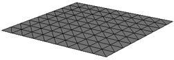
ClothUv Example for Cloth Object dynamics node
This is an example that shows how you can specify the warped and weft directions on a triangulated cloth planel using uv coordinates.
Because the uv directions are aligned with the xy directions of the grid, the result looks nearly identical to a quad grid, even though the mesh is triangulated.
The little blue and yellow lines visualize the directions of the cloth fabric. This is enabled in the Visualization tab of both cloth objects.
DragCloth Example for Cloth Object dynamics node
This example shows how adding Normal and Tanget Drag to a cloth object can influence its behaviour.
MultipleSphereClothCollisions Example for Cloth Object dynamics node
This example shows a pieces of cloth with different properties colliding with spheres. By adjusting the stiffness, bend, and surfacemassdensity values, we can give the cloth a variety of different behaviours.
PanelledClothPrism Example for Cloth Object dynamics node
This example demonstraits a paneling workflow to create a open-ended rectangular prism which keeps its shape.
PanelledClothRuffles Example for Cloth Object dynamics node
This example demonstraits a paneling workflow and use of the seamangle primitive attribute to create a cloth ruffle attached to a static object.
| See also |