| On this page | |
| Since | 12.0 |
The Pyro solver is an extension of the ![]() Smoke Solver. If you just want to generate smoke without combustion (flames), you might consider using the Smoke Solver since it’s a little simpler, however the Pyro solver is more flexible.
Smoke Solver. If you just want to generate smoke without combustion (flames), you might consider using the Smoke Solver since it’s a little simpler, however the Pyro solver is more flexible.
See [how to use the Pyro tools for information on creating simulations using the shelf tools. See Pyro look development for information on using the parameters to achieve different flame and smoke looks.
Setting up 
If you use the shelf tools to create Pyro effects, they will set up the sourcing, solver, and output object for you automatically.
If you are setting up a pyro network from scratch, you can use the ![]() Smoke Object node to create a DOP object with the data required by the Pyro solver already attached. If you already have a DOP object, you can use the
Smoke Object node to create a DOP object with the data required by the Pyro solver already attached. If you already have a DOP object, you can use the ![]() Smoke Configure Object node to add the necessary data to it.
Smoke Configure Object node to add the necessary data to it.
This solver makes use of various field subdata on the object.
-
The object should have a scalar field
densityfor the density of the smoke. -
The object should have a vector field
velfor the velocity at each voxel. -
Optionally, the object can have a scalar field
temperaturefor internal buoyancy calculations.
Inputs 
Object
A ![]() Smoke object to work on. Note that a smoke
object can contain multiple containers.
Smoke object to work on. Note that a smoke
object can contain multiple containers.
Pre-solve
Run the network branch attached to this input before each solving
step. In the standard pyro setup, the attached node (![]() Gas Resize Fluid Dynamic) automatically resizes the fluid containers at each step.
Gas Resize Fluid Dynamic) automatically resizes the fluid containers at each step.
Velocity update
Nodes attached to this input can edit the simulation network’s velocity fields, for example to apply custom forces, before the “project gas non-divergent” step (see also the “Sourcing (post-solve)” input below).
Advection
Connect a ![]() Gas Advect node to this input to allow the it to advect the points of geometry data attached to the container based on the fields in this solver.
Gas Advect node to this input to allow the it to advect the points of geometry data attached to the container based on the fields in this solver.
Sourcing (post-solve)
The main use for this input is to add volumes attached to this input as fuel sources, density sources, sinks, collision fields, pumps, etc. This will usually be done by a ![]() Volume Source node that imports volumes from a geometry network. See pyro sourcing for more information.
Volume Source node that imports volumes from a geometry network. See pyro sourcing for more information.
Nodes attached to this input can also edit the simulation network’s velocity fields, for example to apply custom forces, after the “project gas non-divergent” step.
Parameters 
Simulation 
These parameters control how the simulation develops over time. See how pyro simulations work for information on how the temperature and velocity fields drive the simulation to a great extent.
Time Scale
A scaling factor for time inside this solver. 1 is normal speed, greater than 1 makes the pyro sim appear sped up, less than 1 makes the pyro sim appear to be in slow motion.
You can use expression functions such as doptime, dopframe,dopsttot, and dopttost to convert between global times and simulation times.
Note
Changing the Time Scale only affects the timestep of the simulation. If adding velocities calculated in SOPs to the simulation for collisions or pumps with the ![]() Volume Source DOP, scale the incoming velocities by
Volume Source DOP, scale the incoming velocities by 1 / timescale to match the timestep of the simulation.
Temperature Diffusion
A Gaussian blur factor on the temperature field. Higher values spread the temperature out more and create a less sharply defined effect and more cooling. For example, a value of 2 will blur the temperature field by a radius of 2 every second.
(The real-world motivation for this parameter is to simulate turbulence at a finer scale than the sim’s resolution, which spreads the field out.)
Cooling Rate
How fast the temperature field cools to zero. A value of 0.9 will decrease the temperature of hot gas by 90% (to 10% of its original value) every second.
Warning
This is the inverse of the Cooling Rate parameter in Houdini 11 and lower versions.
Viscosity
The “fluid-ness” of the velocity field. Higher values make neighboring voxels have the same velocity, creating a more flowing look. A value of 0 allows adjacent voxels to move any direction without resistance, creating a more chaotic, turbulent look.
(Inside the solver, higher viscosity values introduce a penalty when a voxel’s velocity varies from that of its neighbors. This is currently implemented by applying a diffusive term to the velocity field.)
Buoyancy Lift
An upward force at each voxel scaled by the difference between the ambient temperature and voxel’s temperature, so hotter areas will get more lift and cooler areas will sink. Increasing this makes the effect rise faster and go higher.
Buoyancy Dir
The direction in which buoyancy is applied. This is usually the Up direction of your simulation, but often can be altered to quickly tweak the look of a sim.
Combustion 
The combustion model takes the fuel field and turns it into burn, temperature, and density (smoke).
Enable Combustion
Enables the combustion model for the Pyro Solver. If this is off, the fuel field and everything else related to burning is ignored.
Ignition Temperature
The combustion model will only occur if the temperature field is above this value. If you want all fuel to instantly ignite, use a negative value.
Burn Rate
The amount of fuel to burn per second. This is a ratio: 0.9 means after one second 90% will be burned.
Fuel Inefficiency
Controls how much of the burned fuel is actually not burned,
but kept. 0 means all burned fuel is removed from the fuel
field. 1 means that no fuel is removed from the fuel field
when it is burnt.
Temperature Output
The amount to increase the temperature field by for every unit of fuel consumed.
This is affected by both the heat and burn fields, as per the influence parameters.
Gas Released
A scale factor controlling how much gas is injected into locations where fuel is burnt. This causes burning areas to blow outwards.
The gas release is scaled by both the heat and burn fields according to the influence parameters.
Flames 
Options controlling the flames (heat).
Flame Height
Scaling factor for flames. Higher values give taller flames, lower values give smaller flames. This value is not measured in any unit (it is not the height of the flames in Houdini units), it simply affects the amount of cooling applied to the flames.
Very low values will not necessarily result in very small flames, since the cooling factor will often not be enough to counteract a hot temperature field.
The inverse of this value (multiplied by the cooling field, see below) is subtracted from the heat field, so lower values give more cooling and smaller flames.
You can use the cooling field controls below to vary the flame height value based on the value in a field (by default the temperature field).
Cooling Field
When enabled, the values in the given field (by default, temperature) are used to vary the flame’s cooling rate across the container.
Cooling field range
The range of values in the control field to map onto cooling amounts.
Remap heat cool field
The ramp’s vertical axis is amount of cooling and the horizontal axis is the value in the control field. For example, the default ramp’s shape, which is high on the left and low on the right, applies more cooling where the temperature is low.
Smoke 
Options controlling the emission of smoke/soot (density).
Emit Smoke
Enables the emission of smoke/soot from burning objects.
Create Dense Smoke
Adds smoke to the system without considering how much smoke is already present. This is good for heavy explosions or big plumes of smoke. When this option is off, smoke is only added up to a certain maximum amount in each voxel, giving a lighter, less dense smoke.
Source
Where the smoke is emitted. The best choice is usually “Heat”, which is more realistic and prevents the smoke from obscuring the flames at source.
Burn
Emit smoke at the point of flame ignition (the burn field) and nowhere else.
Heat
Emit smoke wherever the flames cool to a certain value.
Smoke Amount
Scales the amount of smoke to be added. The base smoke value depends on the value in the field set by the Source parameter (burn or heat).
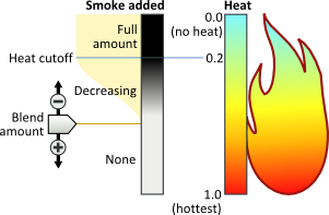
Heat Cutoff
The value of the heat field at which smoke is emitted. This option is only available when Source is “Heat”. For example, if Heat cutoff is 0.2, smoke appears where the heat field is 0.2 or cooler. The Blend amount parameter controls what happens above the heat cutoff point.
Blend Amount
Increasing this parameter gives a smoother fire-to-smoke transition by adding a falloff above the Heat Cutoff value. This option is only available when Source is “Heat”.
The value controls the blend between the full amount of smoke being added at and below the Heat cutoff, and no smoke being added at the highest heat (1.0). A value of 0 adds no smoke above the heat cutoff. A value of 1 blends from adding full smoke at the cutoff point, through decreasing amounts of smoke at higher heat values, up to the highest heat.
Gas 
Options controlling the injection of gas (or expansion in the velocity field).
Flame Contribution
The amount of gas emitted from the flames (the heat field). Increasing this value will blow outwards more strongly in areas where flames are present.
Burn Contribution
The amount of gas emitted from ignition (the burn field). Increasing this value will blow outwards more strongly where fuel is being burned.
Temperature 
Options controlling the emission of temperature from flames and/or ignition.
Flame Contribution
The amount of temperature emitted from flames (the heat field). Increasing this value will make the air hotter in areas with flames.
Burn Contribution
The amount of temperature emitted from ignition (the burn field). Increasing this value will make the air hotter where fuel is being burned.
Fuel 
Options controlling the influence of fuel.
Advect Fuel
When this option is off (the default), fuel is stationary and is not affected by the velocity field. When this option is on, the fuel field as advected just like temperature, heat, and density. Turning this option on makes results more unpredictable and is also slower to calculate.
Fuel Speed
The maximum speed at which fuel can move by advection.
Shape 
The parameters on this tab control the shape and development of the flame/smoke. All except dissipation affect the velocity field as internal forces.
Remember that the resolution of the ![]() Smoke object determines how much detail you can get in the fire/smoke. However, the pyro solver is largely resolution independent, so you can often work in low resolution and then bump up the resolution with similar, more detailed results.
Smoke object determines how much detail you can get in the fire/smoke. However, the pyro solver is largely resolution independent, so you can often work in low resolution and then bump up the resolution with similar, more detailed results.
Houdini includes two different ways to add turbulent noise to fire: shredding and turbulence.
-
Shredding is the main way to add “high frequency” noise to flames. It squashes and stretches the velocity field to create the licks and flows typical of fire.
-
You should use the turbulence to add “low frequency” noise: rolling, churning, large-scale motion.
For each shaping parameter, there is a checkbox to turn the shaping type on, and a scaling factor to control how much of the shaping type to apply, and below those parameters are tabs containing control and visualization parameters for each shaping type.
Expert users: The Pyro solver is implemented using the ![]() Smoke solver with additional subsolvers to provide
Smoke solver with additional subsolvers to provide ![]() Gas Sharpening,
Gas Sharpening, ![]() Confinement,
Confinement, ![]() Shredding,
Shredding, ![]() Turbulence, Dissipation, and
Turbulence, Dissipation, and ![]() Disturbance.
Disturbance.
Note
You can attach additional velocity field updating DOPs such as ![]() Vortex Equalizer,
Vortex Equalizer, ![]() Gas Wind Dop and
Gas Wind Dop and ![]() Gas Damp Dop to the Pyro solver’s second input (“velocity update”).
Gas Damp Dop to the Pyro solver’s second input (“velocity update”).
Dissipation
Causes smoke (density) to disappear over time. Low values cause smoke to disappear slowly, high values cause smoke to disappear quickly.
For example, a value of 0.1 means 10% of the smoke will disappear every twenty-fourth of a second. A value of 1 will make all smoke disappear immediately.
See the Dissipation tab below.
Disturbance
Introduces detail of a certain size in the smoke or fire without changing the general motion or shape of the simulation.
See the Disturbance tab below.
Shredding
Pushes and pulls the velocity field based on gradient of the heat field to create the streaks, separation, and “licks” typical of fire.
Very high values tend to give a random, fractal look, while very low values or no shredding gives blobby flames without much character.
Since shredding works on the gradient of the temperature field, lower temperature diffusion results in a more noticeable shred effect. When temperature diffuses more, the gradient becomes less dynamic, resulting in bigger streaks. The higher the grid resolution, the more detailed the gradient becomes.
See the Shredding tab below.
Turbulence
Adds “churning” noise to the velocity field. You should generally use this to add powerful, large-scale/low-frequency noise and rely on shredding for smaller features. This is especially useful when you have a very fast-moving fire and you want to add more character to it.
See the Turbulence tab below.
Confinement
Boosts swirls (vortices) where they exist, increasing “curliness” in the simulation that would otherwise be lost by the grid resolution. Too high values can make the simulation unstable and blow up. Negative values suppress vortices and smooth out the simulation, but it is usually better to just use a lower resolution grid.
(The Pyro solver does not use explicit vorticles, it can detect vortex locations directly in from the velocity field.)
You can use a ramp to remap the amount of confinement based on the curl amount, for example to apply more confinement to larger vortices.
See the Confinement tab below.
Dissipation 
Control field
When enabled, the force exerted is scaled by the content of this field.
Control range
Map from this range of values in the control field.
Remap dissipation field
The ramp’s vertical axis is amount of dissipation and the horizontal axis is the value in the control field. For example, the default ramp’s shape, which is high on the left and low on the right, makes smoke disappear more quickly where the temperature is low.
Disturbance 
Field To Disturb
The field to apply the disturbance forces to.
Cutoff
Ignore voxels with values higher than this in the “threshold field” (density by default, you can change the field on the Bindings tab). This lets you only affect the edges of the smoke.
Use Block Size
When this option is on, use the Block size parameter to set the size of disturbance elements in word space units. When this option is off, use Locality to control the size of disturbance elements in voxels. Using block sizes avoids issues if you scale the container.
Block Size
Size in world units of the details added. Higher values give larger disturbance elements. Available when Use block size is on.
Locality
Number of voxels are sampled into a certain disturbance value. Higher values give larger disturbance elements. Available when Use block size is off.
Control settings 
Control Field
When enabled, the force exerted is scaled by the content of this field.
Control Influence
A scaling factor on the control field’s influence on the effect. A value of 0 makes the field have no influence.
Control Range
Map from this range of values in the control field.
Remap Control Field
Enables or disables the control field ramp.
Control Field Ramp
The ramp’s vertical axis is strength of the effect and the horizontal axis is the value in the control field.
Bindings 
Threshold Field
Voxels with values higher than the value of the Cutoff parameter in this field will not be disturbed.
Shredding 
Temperature threshold
At temperatures lower than this value the velocity field will be stretched, at temperatures higher than this the velocity will be squashed. Lower values give more shredding at the edges of the flame, where the temperature is lower.
Threshold width
The width of an area around the Temperature threshold where squash and stretch are blended. Lower values give harsher squash and stretch, higher values give smoother streaks.
Squash
How much to squash the velocity field when the temperature is above the Temperature threshold.
Stretch
How much to stretch the velocity field when the temperature is below the Temperature threshold.
Clip gradient
Clips the calculated temperature gradient to this maximum value. This is useful when a simulation has very high temperatures (for example, an exploding fireball) to keep the high temperatures from translating into extreme, bizarre shredding.
Control settings 
The controls on this tab let you vary the amount of shredding across the container based on the values in a field.
Control Field
When enabled, the force exerted is scaled by the content of this field.
Control Influence
A scaling factor on the control field’s influence on the effect. A value of 0 makes the field have no influence.
Control Range
Map from this range of values in the control field.
Remap Control Field
Enables or disables the control field ramp.
Control Field Ramp
The ramp’s vertical axis is strength of the effect and the horizontal axis is the value in the control field.
Visualization 
Visualize shredding
Turn this on to see a viewport visualization of the forces applied to the velocity field by this effect.
See the ![]() Scalar Field Visualization and
Scalar Field Visualization and ![]() Vector Field Visualization node help for information on the visualization parameters.
Vector Field Visualization node help for information on the visualization parameters.
Bindings 
Do not change the values on this tab unless you really know what you're doing.
Sharpness 
Field name
The name of the field to sharpen (usually density, which represents smoke).
Locality
The number of voxels the solver samples when sharpening. When sharpening, small disconnected blobs of cloud can be “sharpened away”. This parameter determines the largest size of blob that can be sharpened away.
Turbulence 
Swirl size
Sets the rough size of the swirls, in Houdini units.
Grain
A scale on the noise added to the swirls with the Turbulence parameter.
Pulse length
The frequency of the noise in time.
Seed
Seeds the random number generator for the noise. Change this number to get different random swirls.
Influence threshold
Turbulence will not apply to voxels with density lower than this value (you can change the field in the Bindings tab). This is largely a performance optimization: the higher you set this value, the faster the turbulence will tend to run because it can skip more voxels.
Turbulence
The amount of noise to add to the swirls.
Control settings 
Control Field
When enabled, the force exerted is scaled by the content of this field.
Control Influence
A scaling factor on the control field’s influence on the effect. A value of 0 makes the field have no influence.
Control Range
Map from this range of values in the control field.
Remap Control Field
Enables or disables the control field ramp.
Control Field Ramp
The ramp’s vertical axis is strength of the effect and the horizontal axis is the value in the control field.
Visualization 
Visualize turbulence
Turn this on to see a viewport visualization of the forces applied to the velocity field by this effect.
See the ![]() Scalar Field Visualization and
Scalar Field Visualization and ![]() Vector Field Visualization node help for information on the visualization parameters.
Vector Field Visualization node help for information on the visualization parameters.
Bindings 
Do not change the values on this tab unless you really know what you're doing.
Confinement 
Control field
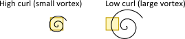
When enabled, the force exerted is scaled by the content of this field. The default control field is confinement, which holds the calculated curl at each voxel (high curl means small vortices).
The Gas Ramp field might also be useful as a control field.
Control Range
Map from this range of values in the control field.
Control Influence
A scaling factor on the control field’s influence on the effect. A value of 0 makes the field have no influence.
Visualization 
Visualize confinement
Turn this on to see a viewport visualization of the forces applied to the velocity field by this effect.
See the ![]() Scalar Field Visualization and
Scalar Field Visualization and ![]() Vector Field Visualization node help for information on the visualization parameters.
Vector Field Visualization node help for information on the visualization parameters.
Control field ramp 
Remap Control Field
Enables or disables the control field ramp.
Control field ramp
The ramp’s vertical axis is amount of confinement and the horizontal axis is the value in the control field. For example, the default ramp’s shape, which is low on the left side and high on the right side, adds more confinement where the curl is high (that is, where the vortices are small).
Bindings 
Do not change the values on this tab unless you really know what you're doing.
Color 
The solver is capable of managing the smoke object’s color data. To this end, it takes care of two
fields: Cd, which stores the color value that can be used as the Diffuse Field for visualization,
and Alpha, which contains the amount of color at each point in space. The Alpha field is important
for determining how colors should be mixed. For example, if white and black smoke mix, the resultant
gray will be lighter if the white component has a higher Alpha value. The clip below provides a
visual comparison: yellow smoke in the right clip is sourced with a larger value of Alpha.
Dissipation
Causes the amount of color (Alpha field) to reduce over time. Note that this does not directly
affect smoke’s color, but makes it easier to mix in new color via sourcing.
Blur
Blurs the smoke’s color field by mixing its values in neighborhoods of the given size.
Sharpening
Sharpens the smoke’s color field, effectively discouraging mixing of different colors.
Note
Large values of the sharpening parameter may introduce visible artifacts. In some cases, the added noise may be reduced by increasing the sharpening Threshold.
Dissipation 
When dissipation is turned on, the amount of color in the smoke reduces over time, making it easier to source new color.
Control Field
When turned on, the amount of dissipation is scaled by the content of this field.
Control Range
Map from this range of values in the control field.
Remap Dissipation Field
The ramp’s vertical axis is amount of dissipation, and the horizontal axis spans Control Range. The default ramp, for example, reduces the amount of color faster in areas where temperature is low.
Blur 
Blur encourages mixing of smoke colors.
Radius
Controls how far out the colors will blur per second.
Filter
Shape of the blur kernel.
Sharpness 
Sharpening fights mixing, helping preserve sharp boundaries between colors.
Radius
Sharpening boosts the deviation of colors from averaged (blurred) values. This parameter controls the distance to which blurring is performed.
Threshold
Sharpening boosts the deviation of colors from averaged (blurred) values. If the deviation falls below this threshold at a voxel, no sharpening is done to it. Increasing this value can help reduce the amount of introduced sharpening noise.
Relationships 
Prior to Houdini 12, the Pyro solver used DOP relationships to associate sources, pumps, sinks, and collision geometry with a fluid container, using the ![]() Merge DOP and/or
Merge DOP and/or ![]() Apply relationship DOP to create the relationship. The preferred method in Houdini 12 and later is to use SOP networks to create sources, pumps, sinks, and collision geometry and import them using the Source volume DOP.
Apply relationship DOP to create the relationship. The preferred method in Houdini 12 and later is to use SOP networks to create sources, pumps, sinks, and collision geometry and import them using the Source volume DOP.
If you want to use the old relationship method to set up sources, sinks, etc., you can enable relationships using the parameters on this tab. By default, relationships are turned off, and the solver ignores relationship data.
You can use both methods (import SOP geometry and attach it to the solver’s “sourcing” input, as well as set up DOP object relationships). When relationships are enabled, the solver will combine the sources, sinks, etc. from both methods.
Enable Relationships
Use object relationship data to add sources, pumps, sinks, and collision geometry to the simulation (in addition to imported data connected to the sourcing input, if any).
Sources 
Tip
When using a source relationship, make sure the source object is emitting temperature. You can set this up on the object’s physical properties tab.
Enable Source Relationship
Use DOP objects with a “source” relationship to the solver.
Add Source To
The field to add the source to. The default is density, which will create smoke. To create flame, you could change this to fuel and set the temperature physical property of the source object.
Source Merge
How the source object’s volume will be added to the simulation. Scale controls the addition amount.
Velocity Merge
How the source object’s velocity will affect the container’s velocity field. Scale controls the amount to add.
Temperature Merge
How the source object’s temperature physical parameter will affect the container’s temperature field. Scale controls the amount of temperature to add.
Velocity Type
How to measure velocity on the source object. If the source geometry does not deform (change shape) over time, use “Rigid velocity”. If the source deforms but does not change topology over time, use “Point velocity”.
Rigid Velocity
Treat the source object as non-deforming.
Point Velocity
Use point history to allow deforming geometry. This only works if the topology of the source geometry doesn’t change.
Volume Velocity
Use the SDF representation of the object. Allows deforming geometry and does not require a fixed topology over time, but cannot detect tangential velocities.
Pumps 
Enable Pump Relationship
Use DOP objects with a “pump” relationship to the solver.
Velocity Merge
How the source object’s velocity will affect the container’s velocity field. Scale controls the amount of velocity to add.
Velocity Type
Temperature Merge
Whether the object’s temperature property affects the temperature field of the container. If you choose “Set interior”, the part of the temperature field corresponding to the inside the object will be set to the object’s temperature.
Collisions 
Enable Collide Relationship
Use DOP objects with a “collision” relationship to the solver.
Temperature Merge
Whether the object’s temperature property affects the temperature field of the container. If you choose “Collision interior”, the part of the temperature field corresponding to the inside the object will be set to the object’s temperature.
Restrict Mask to Bandwidth
Normally the collision mask SDF is only calculated up to a certain distance from the original collision geometry. Turn this off to compute the full range of the mask if you need it for some special effect, such as having things react before they reach the object.
Use Point Velocity for Collisions
Turn this on if the collision geometry is deforming (changing shape) over time, but has consistent topology (e.g. number of points). If the topology changes over time, turn on Use volume velocity for collisions.
Use Volume Velocity for Collisions
Turn this on if the collision geometry is deforming (changing shape) and topology (e.g. number of points) over time.
Collide with Non-SDF
Allows the fluid to collide with objects that don’t have Geometry/SDF, such as other fluids.
Extrapolate into Collisions
Copies the density and fuel fields into the collision field. This causes the smoke to become “sticky” to avoid an air gap between the smoke and the collision field. This also prevents smoke from passing through moving collision fields.
Sink 
Enable Sink Relationship
Use DOP objects with a “sink” relationship to the solver.
Advanced 
You should generally not need to change these parameters.
Use OpenCL
Enable GPU acceleration on certain microsolvers. This may not work on all graphics cards or operating systems. Check the System Requirements information in the Support section of the Side Effects Software website.
You should have a fairly recent graphics card and fully updated drivers. Start with a low resolution test simulation (for example, a 643 grid) to verify that it runs with OpenCL, then try increasing the resolution. The additional memory-transfer overhead of using OpenCL will only become worth it at high resolutions, around 2563.
With the plain smoke solver, simulation after the first frame sourcing will use the GPU. If you add a microsolver that isn’t GPU-enabled, Houdini does the GPU required CPU copying instead of raising an error.
For fastest speeds, the system needs to minimize copying to and from the video card. The example file demonstrates several methods for minimizing copying. See the OpenCL smoke example file for an explanation of how to set up a fast simulation using GPU acceleration.
A very high-resolution plain smoke solver simulation should be faster with OpenCL. However, default Pyro effects will not automatically simulate faster.
-
They tend to be very low resolution for fast initial playback, so they don’t have enough voxels for the GPU acceleration to greatly exceed the overhead.
-
They have a lot of non-GPU shaping nodes. While many nodes are GPU-enabled (such as vortex confinement), quite a few Pyro nodes are based on VOPs and are not GPU-enabled.
-
Caching is enabled by default in DOPs.
-
Resizing is enabled by default. Resizing has to go through the CPU to manage the field changes. It can also fragment the GPU memory resulting in out-of-memory errors.
Min Substeps
Forces the solver to run a minimum number of substeps. Normally the pyro solver works best with no substeps. If you have smoke and unusual forces, you may want to increase this parameter for better stability. Increasing this parameter will usually make the simulation much slower.
Max Substeps
Forces the solver to not run more substeps than this maximum. Normally the pyro solver works best with no substeps. If you have smoke and unusual forces, you may want to increase this parameter for better stability. Increasing this parameter will usually make the simulation much slower.
CFL Condition
When Max Substeps is greater than 1, the solver uses this parameter to decide the number of substeps. The “condition” is that no substep can allow objects to interpenetrate by more than this many voxels. Higher values allow a substep to move smoke by more voxels, possibly letting it pass through collision objects.
Quantize to Max Substeps
When turned on, use substeps that divide up the frame by Max Substeps so that the time always lands on a multiple of 1/Max Substeps.
Frames Before Solve
Delays the actual simulation this many frames after object creation. Sourcing will still occur in these frames. This may be needed if some solve nodes cannot be processed before certain initial conditions have been met.
External Forces 
Scaled Forces
A list of forces to scale by the value of the forcescale field at each voxel. The default is all forces except gravity.
Absolute Forces
A list of forces to apply uniformly to all voxels, ignoring the forcescale field.
Rest Field 
Enable Rest
Creates rest fields, which can be used to track the position of the fluid over time. Turn this on to correctly map noise or textures in the volume shader.
Dual Rest Fields
Creates a rest2 field that is one back from the main rest field, allowing you to run long simulations without popping.
Frames Between Solve
Number of frames before resetting the rest field.
Frame Offset
Which frame the rest field will be reset on. If you are prerolling the simulation, delaying the rest field initialization until after the preroll will usually give a better result.
Time Scale
How fast the rest field moves in response to the velocity field. A value of 1 would make the rest field match the fluid exactly, however that would quickly smear the rest field out in streaks. Values lower than 1 move the rest field slower than the actual fluid, decreasing streaking.
Projection 
The “project non-divergent” step of the simulation removes the divergence components in the velocity field.
Projection Method
The project non-divergence algorithm. “PCG” has more accurate boundary conditions and avoids computation inside collision objects. Multigrid is significantly faster, especially on large or high resolution containers.
Note
PCG is only used for face-sampled velocity fields. If set to center-sampled, a different relaxation method is used. For center-sampled, multigrid should always be used.
Multigrid Iterations
The multigrid project non-divergence method has inaccurate boundary enforcement. You can increase this number to run the enforcement/projection multiple times, making it more accurate. You should not have to set this higher than 5.
Advection 
Advection Type
The algorithm to use for advecting the fields.
Single stage
Equivalent to the ![]() Gas Advect DOP, where each point is back traced through the velocity field once to find the new voxel value.
Gas Advect DOP, where each point is back traced through the velocity field once to find the new voxel value.
BFECC and Modified MacCormack
Run a second basic advection stage, resulting in a sharper fluid that doesn’t disperse as much.
Clamp Values
The error correction of the BFECC and Modified MacCormack advection types can move voxel values outside the container, leading to strange effects such as negative density values. This parameter lets you choose a method to avoid this problem. The default is “Revert”.
None
Do not attempt to prevent error correction from moving values outside the container.
Clamp
Restrict each voxel to the range of values possible given its eight original values.
Revert
If the error-corrected voxel is out of range, return it to the single-stage value.
Reverting can avoid checker artifacts where the error correction breaks down.
Blend
Apply a smooth blend between non-clamped and clamped values as the advected field approaches the clamping limit. Particularly with the Revert option, applying a small amount of Blend (e.g. 0.05 - 0.1) can reduce grid artifacts in the advected field at the cost of some additional smoothing of the field.
Vel Advection Type
The algorithm to use for advecting the velocity field. Higher types in the list will reduce the apparent viscosity of the field, but may add energy or cause chatter.
Advection Method
Controls particle tracing.
Single step
Takes the velocity at each voxel and makes a single step in that direction for the time step. This is fastest and is independent of the speed of the velocity field, but will start to break up for large time steps.
Trace
Ensures the backtracking does not move more than a single voxel before its velocity is updated, allowing for larger time steps.
Trace Midpoint
Like Trace but uses second order advection for more accuracy but slower simulation.
HJWENO
A non-lagrangian integrator, this allows for theoretically more accurate advection of divergent fields. Unfortunately, if too large substeps are taken, it will explode.
Upwind
A faster but less accurate non-lagrangian integrator.
Trace RK3
Like Trace but uses third order advection for more accuracy but slower simulation.
Trace RK4
Like Trace but uses fourth order advection for more accuracy but slower simulation.
Advection CFL
When tracing the particles, this controls how many voxels the particles can move in a single iterations. Higher values give faster tracing and faster advection, but more errors.
Time Scale 
Burn Influence
The amount the solver’s Time Scale parameter affects the burn model. You should leave this set to 0, since the burn model field calculations don’t scale well and can give unexpected results when changed.
Heat Influence
The amount the solver’s Time Scale parameter affects the flame height. This parameter compensates for the natural flame loss caused when you change the solver’s Time Scale. Setting this to 1 will correctly scale the flames as Time Scale changes, but the flames will be smaller.
Collisions 
Correct Collisions
Sets the specified fields to 0 inside collision objects, which helps prevent leaking through moving objects.
Fields to Correct
When Correct Collisions is turned on, fields in this list will have a correction applied inside collision objects.
Feedback Scale
A scale factor for applying feedback forces to other objects. Setting this to 0 will prevent any feedback.
Clear 
Fields to Clear
Zeros out the specified types of fields after the solve step. This ensures the .sim files, which store the complete state of the simulation, do not have extra information, reducing their size and saving time.
None
Do not clear fields.
Static
Clear fields not needed for next time step. Some of these fields will have guides and the guides will start showing zero values since the underlying field was cleared.
Additional
A space separated list of fields to clear after each solve.
Outputs 
First Output
The operation of this output depends on what inputs are connected to this node. If an object stream is input to this node, the output is also an object stream containing the same objects as the input (but with the data from this node attached).
If no object stream is
connected to this node, the output is a data output. This data
output can be connected to an ![]() Apply Data DOP,
or connected directly to a data input of another data node, to
attach the data from this node to an object or another piece of
data.
Apply Data DOP,
or connected directly to a data input of another data node, to
attach the data from this node to an object or another piece of
data.
Locals 
channelname
This DOP node defines a local variable for each channel and parameter on the Data Options page, with the same name as the channel. So for example, the node may have channels for Position (positionx, positiony, positionz) and a parameter for an object name (objectname).
Then there will also be local variables with the names positionx, positiony, positionz, and objectname. These variables will evaluate to the previous value for that parameter.
This previous value is always stored as part of the data attached to the object being processed. This is essentially a shortcut for a dopfield expression like:
dopfield($DOPNET, $OBJID, dataName, "Options", 0, channelname)
If the data does not already exist, then a value of zero or an empty string will be returned.
DATACT
This value is the simulation time (see variable ST) at which the current data was created. This value may not be the same as the current simulation time if this node is modifying existing data, rather than creating new data.
DATACF
This value is the simulation frame (see variable SF) at which the current data was created. This value may not be the same as the current simulation frame if this node is modifying existing data, rather than creating new data.
RELNAME
This value will be set only when data is being attached to a relationship (such as when Constraint Anchor DOP is connected to the second, third, of fourth inputs of a Constraint DOP).
In this case, this value is set to the name of the relationship to which the data is being attached.
RELOBJIDS
This value will be set only when data is being attached to a relationship (such as when Constraint Anchor DOP is connected to the second, third, of fourth inputs of a Constraint DOP).
In this case, this value is set to a string that is a space separated list of the object identifiers for all the Affected Objects of the relationship to which the data is being attached.
RELOBJNAMES
This value will be set only when data is being attached to a relationship (such as when Constraint Anchor DOP is connected to the second, third, of fourth inputs of a Constraint DOP).
In this case, this value is set to a string that is a space separated list of the names of all the Affected Objects of the relationship to which the data is being attached.
RELAFFOBJIDS
This value will be set only when data is being attached to a relationship (such as when Constraint Anchor DOP is connected to the second, third, of fourth inputs of a Constraint DOP).
In this case, this value is set to a string that is a space separated list of the object identifiers for all the Affector Objects of the relationship to which the data is being attached.
RELAFFOBJNAMES
This value will be set only when data is being attached to a relationship (such as when Constraint Anchor DOP is connected to the second, third, of fourth inputs of a Constraint DOP).
In this case, this value is set to a string that is a space separated list of the names of all the Affector Objects of the relationship to which the data is being attached.
ST
The simulation time for which the node is being evaluated.
Depending on the settings of the ![]() DOP Network
Offset Time and Scale Time parameters,
this value may not be equal to the current Houdini time
represented by the variable T.
DOP Network
Offset Time and Scale Time parameters,
this value may not be equal to the current Houdini time
represented by the variable T.
ST is guaranteed to have a value of zero at the
start of a simulation, so when testing for the first timestep of a
simulation, it is best to use a test like $ST == 0, rather than
$T == 0 or $FF == 1.
SF
The simulation frame (or more accurately, the simulation time step number) for which the node is being evaluated.
Depending on the settings of the ![]() DOP Network parameters,
this value may not be equal to the current Houdini frame number
represented by the variable F. Instead, it is equal to
the simulation time (ST) divided by the simulation timestep size
(TIMESTEP).
DOP Network parameters,
this value may not be equal to the current Houdini frame number
represented by the variable F. Instead, it is equal to
the simulation time (ST) divided by the simulation timestep size
(TIMESTEP).
TIMESTEP
The size of a simulation timestep. This value is useful for scaling values that are expressed in units per second, but are applied on each timestep.
SFPS
The inverse of the TIMESTEP value. It is the number of timesteps per second of simulation time.
SNOBJ
The number of objects in the simulation. For nodes that
create objects such as the ![]() Empty Object DOP,
SNOBJ increases for each object that is evaluated.
Empty Object DOP,
SNOBJ increases for each object that is evaluated.
A good way to guarantee unique object names is to use an expression
like object_$SNOBJ.
NOBJ
The number of objects that are evaluated by the current node during this timestep. This value is often different from SNOBJ, as many nodes do not process all the objects in a simulation.
NOBJ may return 0 if the node does not
process each object sequentially (such as the ![]() Group
DOP).
Group
DOP).
OBJ
The index of the specific object being processed by the node. This value always runs from zero to NOBJ-1 in a given timestep. It does not identify the current object within the simulation like OBJID or OBJNAME; it only identifies the object’s position in the current order of processing.
This value is useful for generating a
random number for each object, or simply splitting the objects into
two or more groups to be processed in different ways. This value
is -1 if the node does not process objects sequentially (such
as the ![]() Group DOP).
Group DOP).
OBJID
The unique identifier for the object being processed. Every object is assigned an integer value that is unique among all objects in the simulation for all time. Even if an object is deleted, its identifier is never reused. This is very useful in situations where each object needs to be treated differently, for example, to produce a unique random number for each object.
This value is also the best way to look up information on an object using the dopfield expression function.
OBJID is -1 if the node does not process objects
sequentially (such as the ![]() Group DOP).
Group DOP).
ALLOBJIDS
This string contains a space-separated list of the unique object identifiers for every object being processed by the current node.
ALLOBJNAMES
This string contains a space-separated list of the names of every object being processed by the current node.
OBJCT
The simulation time (see variable ST) at which the current object was created.
To check if an object was created
on the current timestep, the expression $ST == $OBJCT should
always be used.
This value is zero if the node does not process
objects sequentially (such as the ![]() Group DOP).
Group DOP).
OBJCF
The simulation frame (see variable SF) at which the current object was created. It is equivalent to using the dopsttoframe expression on the OBJCT variable.
This value is zero if the node does not process objects
sequentially (such as the ![]() Group DOP).
Group DOP).
OBJNAME
A string value containing the name of the object being processed.
Object names are not guaranteed to be unique within a simulation. However, if you name your objects carefully so that they are unique, the object name can be a much easier way to identify an object than the unique object identifier, OBJID.
The object name can
also be used to treat a number of similar objects (with the same
name) as a virtual group. If there are 20 objects named “myobject”,
specifying strcmp($OBJNAME, "myobject") == 0 in the activation field
of a DOP will cause that DOP to operate on only those 20 objects.
This value is the empty string if the node does not process objects
sequentially (such as the ![]() Group DOP).
Group DOP).
DOPNET
A string value containing the full path of the current DOP network. This value is most useful in DOP subnet digital assets where you want to know the path to the DOP network that contains the node.
Note
Most dynamics nodes have local variables with the same names as the
node’s parameters. For example, in a ![]() Position DOP,
you could write the expression:
Position DOP,
you could write the expression:
$tx + 0.1
…to make the object move 0.1 units along the X axis at each timestep.
Examples 
BillowyTurbine Example for Pyro Solver dynamics node
This example uses the Pyro Solver and a Smoke Object which emits billowy smoke up through a turbine (an RBD Object). The blades of the turbine are created procedurally using Copy, Circle, and Align SOPs.
| See also |