| On this page |
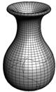
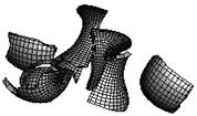
The RBD Fractured Object DOP creates multiple ![]() RBD Object inside the DOP simulation. It takes the geometry from the given SOP Path and breaks it into pieces according to the Group Mask.
RBD Object inside the DOP simulation. It takes the geometry from the given SOP Path and breaks it into pieces according to the Group Mask.
Note
The RBD Fractured Object will make one object for each group. If you have meta groups such as inside and outside, try using piece* instead of *.
Using RBD Fractured Objects 
-
Select the geometry to convert to an RBD fractured object.
-
Define the pieces to be fractured. For example, using the
 Shatter tool.
 -
Select the object and click the
 RBD Fractured Object tool on the Rigid Bodies tab.
 -
Choose whether to use an
 RBD Packed Object or an RBD Fractured Object.
RBD Packed Objects are useful for large simulations since they are much faster, use less memory, and are smaller to write to disk. They can also be influenced by POP Forces, such as drag. Packed Objects can not interact with other solvers such as cloth and fluids. They also only work with Constraint Networks.
Note
Once you convert geometry to an RBD fractured object you can only transform, rotate, and scale it when it is on the first frame.
Attributes 
You can create attributes on the RBD object’s geometry to influence its behavior. Most of these attributes allow fine-tuning of the RBD by overriding default values set in this node.
| Name | Class | Type | Description |
|---|---|---|---|
| v | Point | Vector |
Defines a per-point velocity. This can either be used to define the initial velocity of an RBD object if Inherit Velocity is selected, or the local deformation of the object is Use Per Point Velocities is turned on. |
| friction | Point | Float |
Defines a per-point friction. This will override the friction set in the physical parms page. |
| dynamicfriction | Point | Float |
Defines a per-point dynamic friction. This will override the dynamic friction set in the physical parms page. |
| bounce | Point | Float |
Defines a per-point bounce value. This will override the bounce value set in the physical parms page. |
| nopointvolume | Point | Integer |
Points with this attribute set to true will not be included in the collision information when point sampling is chosen. |
| noedgevolume | Vertex | Integer |
Edges with this attribute set to true will not be included in the collision information when edge sampling is chosen. |
Parameters 
Creation Frame Specifies Simulation Frame
Determines if the creation frame refers to global Houdini
frames ($F) or to simulation specific frames ($SF). The
latter is affected by the offset time and scale time at the
DOP network level.
Creation Frame
The frame number on which the object will be created. The object is created only when the current frame number is equal to this parameter value. This means the DOP Network must evaluate a timestep at the specified frame, or the object will not be created.
For example, if this value is set to 3.5, the
Timestep parameter of the DOP Network must be changed to
1/(2*$FPS) to ensure the DOP Network has a timestep at frame
3.5.
SOP Path
The path to a SOP (or an Object, in which case the display SOP is used) which will be the geometry for this object.
Fracture By Name
The SOP’s geometry is divided into one or more sub-objects. For every unique value of the name attribute, a sub-object will be created with only the primitives that have that attribute value.
Group Mask
The SOP’s geometry is divided into one or more sub-objects. For every group that matches this mask, a sub-object will be created with only the primitives that belong to that group.
Use Deforming Geometry
Causes the geometry for the object to be pulled from the chosen SOP at each timestep. If the SOP contains animated geometry, the RBD object’s geometry will also animate.
If this option is used, the Use Point Velocity parameter of the RBD Solver should also be turned on to take into account the deformations when calculating collision responses.
Re-evaluate SOPs to Interpolate Geometry
Normally when a solver asks for geometry data in a sub-step, the simulation will simply linearly interpolate position data from integral frames. However, this is not exact. Turning this option on re-evaluates the geometry network for each substep. This is more accurate, but can be very expensive.
Use Object Transform
The transform of the object containing the chosen SOP is applied to the geometry. This is useful if the initial location of the geometry is defined by an object transform.
If you want to transfer an object whose movement is defined at the object level, you should use the Object Position DOP instead.
Create Active Objects
Sets the initial active state of the objects. An inactive object doesn’t react to other objects in the simulation.
Display Geometry
Controls if the geometry is displayed in the viewport. Does not reset the simulation when it is changed.
Initial State 
Position
Initial position in world space of the object.
Rotation
Initial orientation of the object. This is in RX/RY/RZ format.
Velocity
Initial velocity of the object.
Angular Velocity
Initial angular velocity of the object. This is the axis of rotation times the rate of rotation. Speed of rotation is measured in degrees per second, so a value of 360 will cause the object to rotate once per second.
Inherit Velocity from Point Velocity
When one brings in a moving piece of geometry from an external source one does not always know the precise velocity and angular velocity.
If this toggle is set, the point velocity attribute of the geometry will be used to calculate the estimated velocity and angular velocity of the object. This allows one to effect a smooth hand off even if the source geometry came from a sequence of geometries rather than a simulation.
Glue 
Glue to Object
The name of an object to glue to. If this is blank, the object is glued to no other object and acts normally. If it is the name of another RBD Object which it mutually affects, this object becomes glued to the other object. Its relative position to the other object is maintained by the solver.
Glue Strength
The amount of accumulated force required to break a glue bond. A value of -1 will prevent the bond from ever breaking. A value of 0 will cause the bond to break with the first external force.
Glue Impulse HalfLife
The number of seconds for the glue impulse to decay by one half. Whenever a glued object gets hit, it accumulates a glue impulse force. This controls how fast that force decays.
Collisions 
Volume 
Use Volume Based Collision Detection
Turning on this option causes the ![]() RBD solver to use a volume
representation of this object for collision detection.
RBD solver to use a volume
representation of this object for collision detection.
The volume representation results in very fast collision detection and very robust results that are tolerant of temporary interpenetrations. The disadvantage is that a volume representation cannot be used to represent a flat object such as a grid, or a hollow sphere.
When this toggle is turned off, the collision detection is geometry-based rather than volume-based. In this case, the collision code will track the trajectories of moving objects over time to find out whether collisions occurred. This allows more accurate results than volume-based collision detection. For this to work, Cache Simulation must be enabled on the DOP network.
Collision Guide
The internal representation used for collision detection is converted to visible geometry. This is useful for debugging problems with collision detection.
This parameter controls the color of the guide geometry.
Mode
Ray Intersect
Use ray intersection with the geometry to create an accurate volumetric representation of the geometry.
Meta Balls
Instead of using rays to determine if points are inside or outside, evaluate the metaball field.
This should be used with Laser Scanning turned off on geometry that consists solely of metaballs.
Implicit Box
Calculate the bounding box for the geometry, and create a volumetric representation that precisely fills that bounding box. This box is always axis aligned in the DOP object’s local space, which is set by the position data.
Note
Use Object Transform bakes the object transform into the geometry’s transform, leaving the Position Data in world space. Turning this off causes the object transform to be send to the Position Data, which causes the object’s local space to be reoriented.
Implicit Sphere
Calculate the bounding sphere for the geometry, and create a volumetric representation that precisely fills that bounding sphere.
Implicit Plane
Calculate the bounding box for the geometry, and create a volumetric representation that divides that box along its smallest axis. Everything below that plane is considered inside, and everything above is outside.
This mode is primarily useful for creating ground planes or immovable walls.
Minimum
Use the distance to the surface or curve. If the Offset Surface is 0, no volume will be made. A positive offset surface will create just that - an offset volume around the object’s surface. This is useful for turning thin objects or wires into actual solids.
Division Method
If Non Square is chosen, the specified size is divided into the given number of divisions of voxels. However, the sides of these voxels may not be equal, possibly leading to distorted simulations.
When an axis is specified, that axis is considered authoritative for determining the number of divisions. The chosen axis' size will be divided by the uniform divisions to yield the voxel size. The divisions for the other axes will then be adjusted to the closest integer multiple that fits in the required size.
Finally, the size along non-chosen axes will be changed to represent uniform voxel sizes. If the Max Axis option is chosen, the maximum sized axis is used.
When By Size is chosen, the Division Size will be used to compute the number of voxels that fit in the given sized box.
Divisions
Controls the creation of the volumetric representation of this object. This should be set fine enough to capture the desired features of the geometry.
Uniform Divisions
The resolution of the key axis on the voxel grid. This allows you to control the overall resolution with one parameter and still preserve uniform voxels. The Uniform Voxels option specifies which axis should be used as the reference. It is usually safest to use the maximum axis.
Division Size
The explicit size of the voxels. The number of voxels will be computed by fitting an integer number of voxels of this size into the given bounds.
Laser Scan
In laser scan mode the volumetric representation is built by sending rays along the primary axes. Only the closest and farthest intersections are used. The space between these two points is classified as inside, and the rest outside.
The laser scan mode will work even with geometry which has poorly defined normals, self intersects, or is not fully watertight. The disadvantage is that interior features can’t be represented as they are not detected.
When laser scanning is turned off, the volumetric representation is still built by sending rays along the primary axes. All intersections are found, however. Each pair of intersections is tested to see if the segment is inside or outside. This relies on the normal of the geometry being well defined (i.e., manifold, no self intersections), and the geometry being watertight. Complicated shapes with holes can be accurately represented, however.
Fix Signs
Even with the best made geometry, numerical imprecision can result in incorrect sign choices. This option will cause the volumetric representation to be post-processed to look for inconsistent signs. These are then made consistent, usually plugging leaks and filling holes.
This takes time, and can be turned off in cases where the volumetric representation is known to generate without problems.
Force Bounds
The Fix Signs method alone will smooth out, and usually eliminate, sign inversions. However, it is possible for regions of wrong-sign to become stabilized at the boundary of the volumetric representation. This option will force all voxels on the boundary to be marked as exterior. The Fix Signs method will be much less likely to stabilize incorrectly then.
Invert Sign
If you want a hollow box, one method is to build one box inside the other and not use Laser Scanning. A more robust method is to just specify the inner box and use sign inversion. This treats everything outside of the box as inside, allowing the more robust Laser Scanning method to be used.
Sign Sweep Threshold
After the fix signs process is complete there can still be inconsistent areas in the SDF. Large blocks can become stabilized and stick out of the SDF. A second sign sweep pass can be performed to try to eliminate these blocks.
The sign sweep threshold governs how big of a jump has to occur for a sign transition to be considered inconsistent. If the values of the sdf change by more than this threshold times the width of the cell, it is considered an invalid sign transition. The original geometry is then ray intersected to determine inside/outside and the result used to determine which sign is correct. The correct sign is then propagated forward through the model.
Max Sign Sweep Count
The sign sweeps are repeated until no signs are flipped (ie, all transitions are within the threshold) or this maximum is reached. Too low of a sign sweep threshold may prevent the process from converging. Otherwise, it tends to converge very quickly.
Offset Surface
A constant amount to offset the signed distance field by. This can be used grow the object slightly or shrink it. Note that it can’t be grown much beyond its original size or it will hit the bounding box of the signed distance field.
Tolerance
This specifies the tolerance used for ray intersections when computing the SDF. This value is multiplied by the size of the geometry and is scale invariant.
File Mode
Controls the operation for this object’s volume data.
Automatic
If a file with the specified name exists already, it is read from disk. Otherwise the volume is created based on the other parameters on this page, and the specified file is created on disk. This file will never be deleted automatically, even when exiting the application.
Read Files
The specified file is read from disk.
Write Files
The volume is created using the other parameters on this page, and is then written to the specified file on disk.
No Operation
The file is never read or written. The parameters on this page are used to create the volume.
File
The name of the file to access according to the choice of File Modes above. This is always .simdata file format. Saving to a .bgeo extension will not save a .bgeo file.
Surface 
Surface Representation
Chooses between colliding points against volume or colliding edges against volume.
Optionally, the point attributes nopointvolume and noedgevolume may be added to the geometry to disable individual points/edges from participating in
collision detection against a volume object. An edge is disabled
if either of its endpoints is disabled.
Convert To Poly
This enables conversion of primitives (such as spheres) in the geometry into polygons. Only polygons are used for collision detection.
Triangulate
When this flag is turned on, polygons in the geometry are triangulated.
LOD
This controls the Level Of Detail of the triangulation. It is used to specify the point density in the U and V directions.
Add Barycenters
The barycenters of each polygon can be included in the collision detection as points or edges (connected to the vertices of the primitive).
Bullet Data 
Show Guide Geometry
When turned on, displays a visualization of the object’s collision shape, including the Collision Padding. This is useful for debugging issues with collision detection, but is typically slower than only displaying the object’s geometry.
Color
The color of the guide geometry.
Deactivated Color
The color of the guide geometry if the object is not moving and has been deactivated by the ![]() Bullet Solver.
Bullet Solver.
Geometry Representation
The shape used by the Bullet engine to represent the object. The Show Guide Geometry parameter can be used to visualize this collision shape.
Convex Hull
The default shape for the object. The ![]() Bullet Solver creates a collision shape from the convex hull of the geometry points.
Bullet Solver creates a collision shape from the convex hull of the geometry points.
Concave
The ![]() Bullet Solver converts the geometry to polygons and creates a concave collision shape from the resulting triangles.
This shape is useful when simulating concave objects such as a torus or a hollow tube. However, it is recommended to only use the concave representation when necessary, since the convex hull representation typically provides better performance.
Bullet Solver converts the geometry to polygons and creates a concave collision shape from the resulting triangles.
This shape is useful when simulating concave objects such as a torus or a hollow tube. However, it is recommended to only use the concave representation when necessary, since the convex hull representation typically provides better performance.
Box
The bounding box of the object.
Capsule
The bounding capsule of the object.
Cylinder
The bounding cylinder of the object.
Compound
Creates a complex shape consisting of Bullet primitives (including boxes, spheres, and cylinders). You will need to use the ![]() Bake ODE SOP.
Bake ODE SOP.
Sphere
The bounding sphere of the object.
Plane
A static ground plane.
Create Convex Hull per Set of Connected Primitives
When turned on, and Geometry Representation is set to Convex Hull, the ![]() Bullet Solver creates a compound shape that contains a separate convex hull collision shape for each set of connected primitives in the geometry.
Bullet Solver creates a compound shape that contains a separate convex hull collision shape for each set of connected primitives in the geometry.
AutoFit Primitive Boxes, Capsules, Cylinders, Spheres, or Planes to Geometry
When turned on, the object’s Geometry subdata is analyzed instead of using the Position, Rotation, Box Size, Radius, and Length values.
When Geometry Representation is set to Box, Capsule, Cylinder, Sphere, or Plane, use the geometry bounds to create the shape.
Position
The position of the object shape in the Bullet world. This parameter is available when Geometry Representation is set to Box, Sphere, Capsule, Cylinder, or Plane, and AutoFit Primitive Boxes, Capsules, Cylinders, Spheres, or Planes to Geometry is turned off.
Rotation
The orientation of the object shape in the Bullet world. This parameter is available when Geometry Representation is set to Box, Capsule, Cylinder, or Plane, and AutoFit Primitive Boxes, Capsules, Cylinders, Spheres, or Planes to Geometry is turned off.
Box Size
The half extents of the box shape. This parameter is available when Geometry Representation is set to Box, and AutoFit Primitive Boxes, Capsules, Cylinders, Spheres, or Planes to Geometry is turned off.
Radius
The radius of the sphere shape. This parameter is available when Geometry Representation is set to Sphere, Capsule, or Cylinder, and AutoFit Primitive Boxes, Capsules, Cylinders, Spheres, or Planes to Geometry is turned off.
Length
The length of the capsule or cylinder in the Y direction. This parameter is available when Geometry Representation is set to Capsule or Cylinder, and AutoFit Primitive Boxes, Capsules, Cylinders, Spheres, or Planes to Geometry is turned off.
Collision Padding
A padding distance between shapes, which is used by the Bullet engine to improve the reliability and performance of the collision detection. You may need to scale this value depending on the scale of your scene. This padding increases the size of the collision shape, so it is recommended to turn on Shrink Collision Geometry to prevent the collision shape from growing.
This parameter is not available when Geometry Representation is set to Plane.
Shrink Collision Geometry
When turned on, shrinks the collision geometry to prevent the Collision Padding from increasing the effective size of the object.
This can improve the simulation’s performance by preventing initially closely-packed collision shapes from interpenetrating, and also removes the gap between objects caused by the Collision Padding.
When Geometry Representation is set to Box, Capsule, Cylinder, Compound, or Sphere, the radius and/or length of each primitive is reduced by Shrink Amount.
When Geometry Representation is set to Convex Hull, each polygon in the representation geometry is shifted inward by Shrink Amount.
This parameter is not available when Geometry Representation is set to Concave or Plane.
Shrink Amount
The amount of resizing done by Shrink Collision Geometry. By default, this value is equal to the Collision Padding so that the resulting size of the collision shape (including the Collision Padding) is the same size as the object’s geometry.
This parameter is not available when Geometry Representation is set to Concave or Plane.
Add Impact Data
When turned on, any impacts that occur during the simulation is recorded in the Impacts or Feedback data. Turning on this option may cause the simulation time and memory usage to increase.
The Impacts and Feedback data are added as subdata on the DOP object. You can see them in the details view when there is at least one impact during the timestep.
The Feedback data is essentially the same as the Impacts data, but is used when there is mutual interaction in the DOP network between multiple objects that are being solved by different solvers. For example, for an RBD object and FLIP fluid object to mutually interact, the DOP network runs multiple feedback loops to resolve the interactions, and the Feedback data is used to pass impact data between the solvers.
Enable Sleeping
When turned on, disables simulation of a non-moving object until the object moves again. The linear and angular speed thresholds are used to determine whether the object is non-moving. If Display Geometry is turned off, you will see the color of the guide geometry change from the Color to the Deactivated Color.
Linear Threshold
The sleeping threshold for the object’s linear velocity. If the object’s linear speed is below this threshold for a period of time, the object may be treated as non-moving.
Angular Threshold
The sleeping threshold for the object’s angular velocity. If the object’s angular speed is below this threshold for a period of time, the object may be treated as non-moving.
Physical 
Compute Mass
Determines if the mass will be calculated automatically from the object’s volumetric representation and glued sub-objects.
Density
The mass of an object is its volume times its density.
Mass
The absolute mass of the object.
Rotational Stiffness
When an object receives a glancing blow, it will often acquire a spin. The amount of spin acquired depends on the shape and mass distribution of the object, known as the inertial tensor.
The Rotational Stiffness is a scale factor applied to this. A higher stiffness will make the object less liable to spinning, a lower value will make it more ready to spin.
Bounce
The elasticity of the object. If two objects of bounce 1.0 collide, they rebound without losing energy. If two objects of bounce 0.0 collide, they come to a standstill.
Bounce Forward
The tangential elasticity of the object. If two objects of bounce forward 1.0 collide, their tangential motion is affected only by friction. If two objects of bounce forward 0.0 collide, their tangential motion is matched.
Friction
The coefficient of friction for the object. A value of 0 means the object is frictionless.
This governs how much the tangential velocity is affected by collisions and resting contacts.
Dynamic Friction Scale
An object sliding may have a lower friction coefficient than an object at rest. This is the scale factor that relates the two. It is not a friction coefficient, but a scale between zero and one.
A value of one means that dynamic friction is equal to static friction. A scale of zero means that as soon as static friction is overcome, the object acts without friction.
Temperature
Temperature marks how warm or cool an object is. This is used in gas simulations for ignition points of fuel or for buoyancy computations.
Since this does not relate directly to any real world temperature scale, ambient temperature is usually considered 0.
Outputs 
First
The RBD objects created by this node are sent through the single output.
Locals 
ST
The simulation time for which the node is being evaluated.
Depending on the settings of the ![]() DOP Network
Offset Time and Scale Time parameters,
this value may not be equal to the current Houdini time
represented by the variable T.
DOP Network
Offset Time and Scale Time parameters,
this value may not be equal to the current Houdini time
represented by the variable T.
ST is guaranteed to have a value of zero at the
start of a simulation, so when testing for the first timestep of a
simulation, it is best to use a test like $ST == 0, rather than
$T == 0 or $FF == 1.
SF
The simulation frame (or more accurately, the simulation time step number) for which the node is being evaluated.
Depending on the settings of the ![]() DOP Network parameters,
this value may not be equal to the current Houdini frame number
represented by the variable F. Instead, it is equal to
the simulation time (ST) divided by the simulation timestep size
(TIMESTEP).
DOP Network parameters,
this value may not be equal to the current Houdini frame number
represented by the variable F. Instead, it is equal to
the simulation time (ST) divided by the simulation timestep size
(TIMESTEP).
TIMESTEP
The size of a simulation timestep. This value is useful for scaling values that are expressed in units per second, but are applied on each timestep.
SFPS
The inverse of the TIMESTEP value. It is the number of timesteps per second of simulation time.
SNOBJ
The number of objects in the simulation. For nodes that
create objects such as the ![]() Empty Object DOP,
SNOBJ increases for each object that is evaluated.
Empty Object DOP,
SNOBJ increases for each object that is evaluated.
A good way to guarantee unique object names is to use an expression
like object_$SNOBJ.
NOBJ
The number of objects that are evaluated by the current node during this timestep. This value is often different from SNOBJ, as many nodes do not process all the objects in a simulation.
NOBJ may return 0 if the node does not
process each object sequentially (such as the ![]() Group
DOP).
Group
DOP).
OBJ
The index of the specific object being processed by the node. This value always runs from zero to NOBJ-1 in a given timestep. It does not identify the current object within the simulation like OBJID or OBJNAME; it only identifies the object’s position in the current order of processing.
This value is useful for generating a
random number for each object, or simply splitting the objects into
two or more groups to be processed in different ways. This value
is -1 if the node does not process objects sequentially (such
as the ![]() Group DOP).
Group DOP).
OBJID
The unique identifier for the object being processed. Every object is assigned an integer value that is unique among all objects in the simulation for all time. Even if an object is deleted, its identifier is never reused. This is very useful in situations where each object needs to be treated differently, for example, to produce a unique random number for each object.
This value is also the best way to look up information on an object using the dopfield expression function.
OBJID is -1 if the node does not process objects
sequentially (such as the ![]() Group DOP).
Group DOP).
ALLOBJIDS
This string contains a space-separated list of the unique object identifiers for every object being processed by the current node.
ALLOBJNAMES
This string contains a space-separated list of the names of every object being processed by the current node.
OBJCT
The simulation time (see variable ST) at which the current object was created.
To check if an object was created
on the current timestep, the expression $ST == $OBJCT should
always be used.
This value is zero if the node does not process
objects sequentially (such as the ![]() Group DOP).
Group DOP).
OBJCF
The simulation frame (see variable SF) at which the current object was created. It is equivalent to using the dopsttoframe expression on the OBJCT variable.
This value is zero if the node does not process objects
sequentially (such as the ![]() Group DOP).
Group DOP).
OBJNAME
A string value containing the name of the object being processed.
Object names are not guaranteed to be unique within a simulation. However, if you name your objects carefully so that they are unique, the object name can be a much easier way to identify an object than the unique object identifier, OBJID.
The object name can
also be used to treat a number of similar objects (with the same
name) as a virtual group. If there are 20 objects named “myobject”,
specifying strcmp($OBJNAME, "myobject") == 0 in the activation field
of a DOP will cause that DOP to operate on only those 20 objects.
This value is the empty string if the node does not process objects
sequentially (such as the ![]() Group DOP).
Group DOP).
DOPNET
A string value containing the full path of the current DOP network. This value is most useful in DOP subnet digital assets where you want to know the path to the DOP network that contains the node.
Note
Most dynamics nodes have local variables with the same names as the
node’s parameters. For example, in a ![]() Position DOP,
you could write the expression:
Position DOP,
you could write the expression:
$tx + 0.1
…to make the object move 0.1 units along the X axis at each timestep.
Examples 
ShatterDebris Example for RBD Fractured Object dynamics node
This example demonstrates the how the shatter, RBD Fractured Object, and Debris shelf tools can be used to create debris emanating from fractured pieces of geometry.
First, the Shatter tool (from the Model tool shelf) is used on the glass to define the fractures. Then the RBD Fracture tool is used on the glass to create RBD objects out of the fractured pieces. Then the Debris tool is used on the RBD fractured objects to create debris.
ShatterGlass Example for RBD Fractured Object dynamics node
This example demonstrates the how the RBD Fractured Object, RBD Pin Contraints, and RBD Material Fracture can be used to shatter glass in Houdini.
StackedBricks Example for RBD Fractured Object dynamics node
This example shows how to create a large number of RBD objects from a single SOP. It also shows how a velocity point attribute can be used to set the initial motion for the objects.
| See also |