| On this page |
Overview 
Sticky collisions allow you to create new constraints with infinite strength to stick objects together when the solver detects an impact. Using this collision method is a good way to avoid artifacts, like objects separating and pulling back again. SOP solvers give you full control over the system’s constraints and their behavior. Various attributes provide valuable information for setting up and customizing your constraint networks. You can also exclude objects from being tagged as sticky, configure the number of collision points, and limit the number of stuck objects.
Sticky collisions are supported in both DOPs and SOPs. In DOP setups, the ![]() Bullet RBD Solver DOP has a Sticky Collisions subpane, where you can specify internal and external constraint networks where new constraints should be generated. These parameters control which constraint network the new constraints should be added to.
Bullet RBD Solver DOP has a Sticky Collisions subpane, where you can specify internal and external constraint networks where new constraints should be generated. These parameters control which constraint network the new constraints should be added to.
Note
Sticky collisions also work well in conjunction with Houdini’s crowd system. For more information, see Ragdoll simulation.
Basic SOP setup 
Sticky collisions are created using an ![]() RBD Configure SOP for basic collision detection. There you can find a Sticky Collisions subpane with various parameters. The system works using a sticky object and a target object. Both names are just definitions to make things distinguishable.
RBD Configure SOP for basic collision detection. There you can find a Sticky Collisions subpane with various parameters. The system works using a sticky object and a target object. Both names are just definitions to make things distinguishable.
A basic network consists of two branches: one for the sticky part and another one for the target. In the end, both branches are merged and connected to a ![]() RBD Bullet Solver SOP solver or a
RBD Bullet Solver SOP solver or a ![]() DOP Network SOP.
DOP Network SOP.
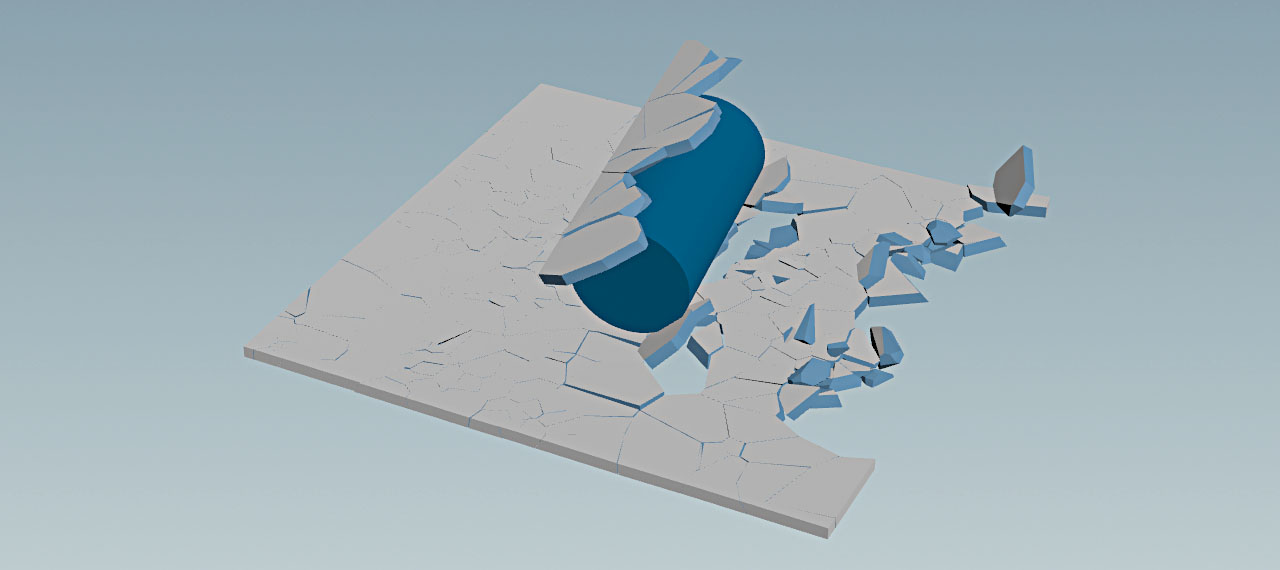
For example, to demonstrate sticky collisions we simulate a cracked ground object (target) that collides with a cylinder (sticky). When the cylinder comes in contact with the ground’s fragments, some pieces will stick to the target object.
Example 
Step 1: Create target object 
The target object is a box that is going to be fractured.
-
Use the
 Box tool on the Create shelf to create a box.
 -
Double-click the
box_object1to dive down to the geometry level. -
Set the box’s Size values to
5,0.1, and5to create a thin glass pane. -
Change the Y value of the Center parameter to
ch("sizey")/2. This expression takes the box’s Scale.Y value and halves it. This makes the box sit directly on the ground plane, no matter how thick it is. We will add a ground plane later.
Step 2: Fracture object 
Houdini provides several methods to fracture objects. The most convenient and realistic approach is using material-based fracturing.
-
Add a
 RBD Material Fracture SOP and connect its first input with the Box SOP’s output.
 -
On the Primary Fracture tab, set Fracture Level to
1to create a less complex fracture pattern. -
In the Cell Points section, increase the Scatter Points to
400to increase the number of pieces. -
In the Fog Volume section, change Noise Frequency to
2,0,2. -
Change the value of Noise Offset to
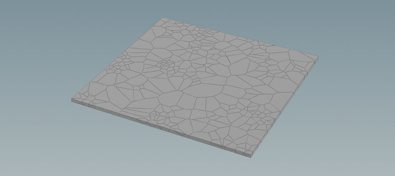
0,0,2. This shifts the cracks along the XYZ axes and will create a more uniform distribution of the fragments. The following image shows the difference between default and modified settings.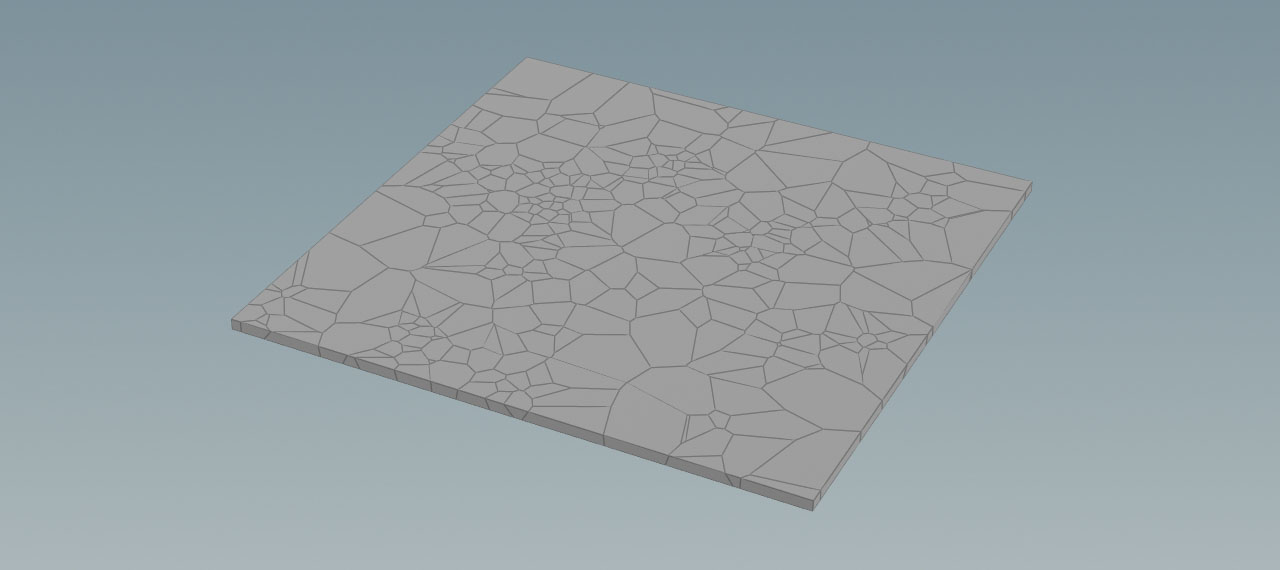
Step 3: Tagging as target object 
In this step, the target object is tagged as a rigid body.
-
Add a
 RBD Configure SOP and connect its first input to the RBD Material Fracture node’s first output.
 -
In the Attributes section, set Name Prefix to
target.
Step 4: Create sticky object 
The sticky object is a tube with some initial linear and angular velocity. The tube rolls over the target cube and collects some glass shards.
-
Put down a
 Tube SOP.
 -
In the Orientation dropdown menu, choose Z Axis.
-
Turn on End Caps to make it a closed cylinder.
-
Use the Center parameters to translate the tube to
3,1.1,0. -
Set the Height to
2. -
Change the value for Columns to
60to create a smoother surface. -
To give the tube some initial velocity, add two
 Attribute Adjust Vector SOP nodes.
 -
Connect input of the first node to the tube’s output.
-
Connect the input of the second node to the first Attribute Adjust Vector SOP’s output.
-
Go to the Attribute Name parameters of the two nodes and enter
vfor the first, andwfor the second node. The attributes stand for linear (v) and angular (w) velocity. -
Set the Constant Value for
vto-5.5,0,0. This makes the tube move in negative X direction. -
Set the Constant Value for
wto0,0,8. This makes the tube spin around its Z axis.
Step 5: Create sticky collisions 
The last node of the sticky branch turns the tube into a rigid body with sticky collisions.
-
Add another
RBD Configure SOP and connect its first input to the output of the last Attribute Adjust Vector node (the node for angular velocity w). -
In the Attributes section, set Name Prefix to
sticky. -
Go to the Sticky Collisions section and turn on Min Sticky Collision Impulse. The impulse relies on substeps and can be a bit tricky to adjust. If the impact is strong enough, the solver adds glue constraints to the constraint network.
-
Change the parameter’s value to
15to make more pieces stick to the tube.
Step 6: Merge branches 
To complete the setup, we must merge the sticky and target branches together for the simulation.
-
Add a
 Merge SOP and connect its input to the first outputs of the RBD Configure SOPs.
 -
Add a
 RBD Bullet Solver SOP, and connect its first output with the Merge SOP’s output.
 -
Go to the Collision tab’s Ground Collision section. From the Ground Type drop-down menu, choose Ground Plane to create an infinite collision plane.
-
Press the
 Play button on the playbar to start the simulation. You should see a result similar to the video below.
 Tip
Try different linear and angular velocities, impulse thresholds, and tube positions to get a feeling for the parameter values.
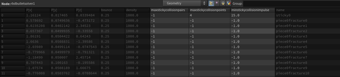
Attributes 
Sticky collisions introduce several new attributes and it can be helpful to monitor them during simulation. The RBD Configure SOP’s Sticky Collisions parameters are also available as point attributes: minstickycollisionimpulse, maxstickycollisionobjects, and maxstickycollisionpoints. Their values correspond directly with the parameter values. To see them in the Geometry Spreadsheet, select the RBD Configure SOP with active sticky collisions, then turn on the Points ![]() mode in the Geometry Spreadsheet.
mode in the Geometry Spreadsheet.
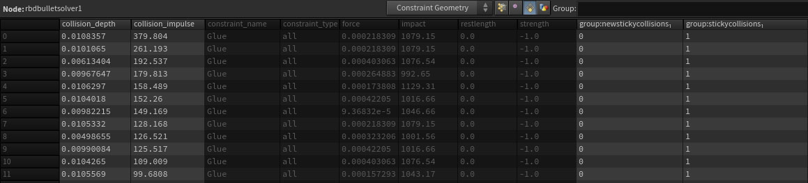
The solver also processes a range of primitive attributes. collision_depth tells you how deep the collision point was inside the surface. newstickycollisions is a primitive group containing the new constraints that were created during the last time step. This is important if you want to use a SOP Solver to control and modify the constraints. stickycollisions is a primitive group containing all of the constraints produced by sticky collisions.
Note
The solver creates these primitive attributes/groups on the constraint geometry when it adds constraints from sticky collisions, not the objects’ geometry.
To monitor these attributes do the following.
-
Select the RBD Bullet Solver SOP.
-
In the Geometry Spreadsheet pane, choose Constraint Geometry from the first drop-down menu.
-
Turn on the Primitives
 mode.
mode.
How to 
| To... | Do this |
|---|---|
|
Control stickiness |
The Min Sticky Collision Impulse parameters determine the minimum impact that is required to make an object stick to the sticky object. Min Sticky Collision Impulse relies on substeps and it can be a bit tricky to find working values. Imagine an object colliding with a wall. With only |
|
Avoid swinging objects |
The solver creates glue constraints by default, which produces a perfectly rigid attachment with one constraint/contact point. However, if you change the constraint type to a soft constraint which allows some motion, they might swing around the constraint’s anchor point when the object hits the surface. To avoid this behavior, increase Max Sticky Collision Points. Higher values add more contact points and constraints. |
|
Exclude objects |
Sticky Collision Ignore accepts objects that will be ignored. The objects can still collide, but won’t stick. This is often necessary if objects should only stick to one character or certain objects (e.g. magnetic vs not magnetic). You can work with object lists, but also wildcards like |
|
Restrict the number of objects sticking to a target |
With Max Sticky Collision Objects you can define how many objects can stick to a target. Imagine you have seven objects colliding with the target, but only three of them should get stuck. A value of |
|
Work with instanced rigid bodies |
The workflow is the same as described in the Basic SOP Setup above. For example, you can scatter objects and configure them as rigid bodies. Then you add a sticky object and let it collide with the scattered instances. |
|
Control the sticky collision constraints' stiffness |
Use a
The following video shows the setup with soft constraints. Notice how the pieces are dragged behind the tube. |
|
Fix misbehaving objects |
|