| On this page |
When loose stones and rocks become unstable, they slide down for a rather short distance and form out deposits in lower areas. The  HeightField Slump COP lets you simulate and fine-tune this process.
The node provides three different modes for creating slump: Smooth, Granular, and Rainfall. The first two modes have almost identical parameter sets and work in the same way. The difference between Smooth and Granular is that the latter mode creates a bumpy surface pattern to the smoothed areas. A seed value lets you redistribute this pattern.
For Smooth and Granular, the Repose Angle plays a central role. This is the maximum angle at which loose material can rest on a slope without sliding down. For example, with 40, material in areas that are steeper than 40 degrees will slide down. With 70, only material in very steep parts will become unstable. With a value of 15, however, almost the entire mountain can slide and you get a very smooth landscape.

Rainfall is a simplified, yet powerful erosion model without simulation. This mode creates channels and gullies similar to hydro erosion. The effect of this mode is often subtle and in many cases you need rather high parameter values to see a result. However, Rainfall is perfectly suited for the creation of creek-like flow maps.
The Debris Scale is relevant for all three modes and describes the size of the eroded material. With higher settings you’ll get a smoother terrain. In conjunction with Rainfall, the parameter defines the width of the erosion gullies. For fine structures, start with a value around 0.01.
Tip
If you want to quickly generate flow maps, please also consider the HeightField Flow Field tool. This is essentially a preconfigured HeightField Slump COP.
Debris input 
You can connect two sources to the node: a terrain on the height input and a supporting debris layer. The debris input can be a mask, for example from the  HeightField Mask by Feature COP. The masks determines, where the eroded material will finally come to rest. As a result you’ll get a typical debris mound around the base of the mountains.
It’s also possible to connect another terrain to the debris input. For example, you can add an already eroded version of the base terrain at the slump node’s height input. This opens completely different possibilities. Or you create a custom image and plug it to the input. The only requirement is that you connect a mono layer.
Flow maps 
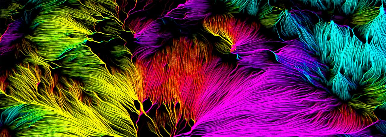
The flow output provides the direction vectors of the slump and visualizes the way, the debris took while sliding down the hill. What you get is a color-coded RGB map that is often used for colorizing or distortion. The following example illustrates how to distort a color map with a flow map from the node’s Rainfall mode. Start with a basic terrain. Feel free to create a more realistic and interesting terrain by adding a  HeightField Erode COP and a HeightField Mask by Feature COP.
-
Add a HeightField Slump COP. Connect the slump node’s
heightinput with theheightornoiseoutput of the previous node. This slump node creates the “base” debris. -
Now, lay down another slump node and connect it (
height→height). -
On the new node, change Slump Mode to Rainfall.
With the second slump you’ll hardly see any difference. The idea is to use a flow map from the rainfall to drive distortion. If you want to see the actual map, connect a  Null COP to the
 flow output of the second slump node. Then, turn on the null node’s blue Display flag and the last slump node’s orange 3D Output flag. The latter flag projects the map onto the actual geometry. Please see 3D Output flag workflow for more information.
-
On the second slump node, set Debris Scale to
0.1to create thinner streams of water.
Colors 
The color network uses the first HeightField Slump COP and the purpose of the second node is to distort the slump. The image shows a preview of the setup because a purely text-based description can be confusing.

The red  Mono to RGB COP starts at the first slump node’s
 height output. For better visibility of the result, all height values are mapped to a Sand ramp color instead of a complex terrain gradient. For a correct distribution, click the Compute Range button. This will add the smallest and largest height values to the Input Min and Input Max parameters.
The blue nodes use the information from the debris output - the actual slump. The  Equalize COP maps the slump color values to a 0-1 range and feeds the processed data to another Mono to RGB COP and a
  Remap COP. The remap node creates an adjustable mask to make the slump visible against the background; the mono node maps the values to pure white.
-
The red Mono to RGB COP goes into the
bginput of a Blend COP.
 -
The blue Mono to RGB COP goes into the
fginput. -
The blue Remap COP goes into the
maskinput.
To finally adjust the amount of visible slump, select the Remap COP, and drag the Threshold slider to the left. Decreasing values reveal more and more slump in the form of white spots.
Distortion 
The last step uses the flow map from the second slump node to distort the white spots. Lay down a  Distort COP. Connect the
 source input with the blend output of the Blend COP. Then, link the dir (direction) input with the flow output of the second slump node. Turn on the distort node’s blue Display flag and the second slump node’s orange 3D Output flag.
To turn the spots into streaks, open then distort node’s Streak dropdown menu and choose Blur. Then increase Scale to stretch the spots along the vectors of the flow map. You should now see a result similar to the image below.
