PDG ML Training Monitor

An interactive real-time data visualization tool for machine learning experimentation

On this page

Overview
Supported nodes
Configuring nodes for the panel
Using the training monitor

Overview ¶

The PDG ML training monitor is a Python panel in Houdini that provides interactive and real-time visualizations of any TOPs ML node.

You can freely switch between different nodes. When the selected node has the correct configuration, the panel will automatically display the relevant information.
You can view training metrics and trends over time using interactive plots based on the data inside a CSV file. These can be a custom file or part of the selected ML node.
When viewing test results, you can see image data generated by the ML node.

Supported nodes ¶

Configuring nodes for the panel ¶

While the panel is built to work out of the box with a list of supported nodes, you can still use it with any other node as long as you configure it correctly. To use the panel, your selected ML node needs an ml_description attribute as part of the node’s HDA module. See HDAModule for more information.

To add the ml_description attribute to your node:

on your node and select Type Properties.
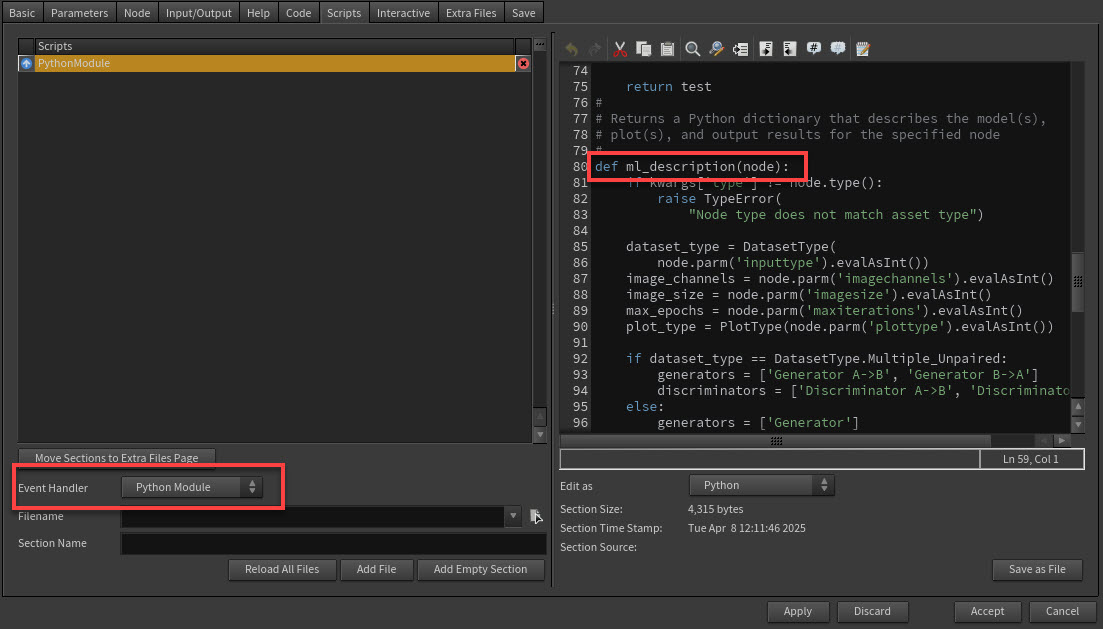
In the Edit Operator Type Properties window, select the Scripts tab.
In the Event Handler dropdown, select Python Module.
In the right side editor, add the function def ml_description(node):
- The ml_description function should return a list of dictionaries with properties. Each node can have multiple ML models which results in each dictionary referring to information about a specific model.

Configuration properties ¶

Property Name	Property Type	Property Value
name	string	The ML model’s name. This field is required.
first_epoch	positive integer	The first epoch number the model starts training from. If this field is unspecified, the default is 0.
max_epochs	positive integer	The maximum number of epochs the model is expected to train for. If this field is unspecified, the default is 500.
plots	list of dictionaries	The information needed for plotting. The keys and values for each dictionary are specified in the Plot Properties table. Each ML model can have multiple plots, so each dictionary corresponds to a different plot. If this field is unspecified, then no plot data will be displayed for this model.
test	dictionary	The information needed for displaying test results in the form of images. The keys and values are specified in the Test Results Properties table. If not provided, then no test data will be displayed for this model.

Plot properties ¶

Property Name	Property Type	Property Value
title	string	The title of the plot. This field is required.
x_axis	string	The label for the x_axis. This field is required.
y_axis	string	The label for the y_axis. This field is required.
x_range	list/tuple	The minimum and maximum values defining the range of the x-axis. To have the range be determined automatically based on the data, leave this null or undefined.
y_range	list/tuple	The minimum and maximum values defining the range of the y-axis. To have the range be determined automatically based on the data, leave this null or undefined.
path_format	string	An absolute path for the CSV file where the plot data is written out. The string provided must not be a template string as the panel will not apply any string formatting. This field is required.

Test results properties ¶

Property Name	Property Type	Property Value
path_format	string	A file path template string for the image file that displays the test results. The named placeholders `{epoch}, {component}, {test}` must be in the path. No other placeholders should be in the path. This is a required field.
count	positive integer	The test size per epoch. In this case, the test size refers to the number of sets of test images. If not provided, then the test size is assumed to be 1. The test numbers themselves are 0-indexed.
rate	positive integer	The interval in epochs at which test results are shown. If not provided, then test results will be displayed every epoch.
components	list of strings	Specifies which images to include in each test result.

Example node configuration ¶

This is an example of an object returned by the ml_description function.

[{'name': 'Generator',
  'first_epoch': 10,
  'max_epochs': 100,
  'plots': [{'title': 'Loss',
             'x_axis': 'Training Progress',
             'y_axis': 'Loss Values',
             'x_range': None,
             'y_range': None,
             'path_format': '/home/user/path/to/csv/loss.csv'},
            {'title': 'SSIM Scores',
             'x_axis': 'Training Progress',
             'y_axis': 'SSIM Score',
             'x_range': None,
             'y_range': (0, 1),
             'path_format': '/home/user/path/to/csv/ssim.csv'}],
  'test': {'path_format': '/home/user/path/to/image/{epoch}.{test}.{component}.png',
           'count': 2,
           'rate': 5,
           'components': ['input', 'reference', 'generated']}},
 {'name': 'Discriminator',
  'first_epoch': 10,
  'max_epochs': 100,
  'plots': [{'title': 'Discriminator Score',
             'x_axis': 'Training Progress',
             'y_axis': 'Score',
             'x_range': None,
             'y_range': (0, 1),
             'path_format': '/home/user/path/to/csv/score.csv'}]}]

Configuring CSV plots ¶

The panel only reads the provided CSV file. This means you must implement the logic that writes the data to the CSV when the node cooks.

The CSV file contents must be in the following format

The first row is the column names, the remaining rows are data.
The data in the first column is the x-axis values.
The data in the other columns are y-axis values, each column represents a separate line in the graph.
Rows cannot have missing data.

This example shows:

x-axis is Epoch
The plot will have 2 lines, one for Generator L1 Loss, and one for Generator Model Loss

Epoch,Generator L1 Loss, Generator Model Loss
0,0.9,0.6
1,0.8,0.5
2,0.7,0.4

Configuring test results ¶

Following the example in the previous section. The results are

rate = 5
first_epoch = 10
max_epochs = 100
path_format = '/home/user/path/to/image/{epoch}.{test}.{component}.png'
count = 2
components = ['input', 'reference', 'generated']

The panel is setup to display every rate images from first_epoch to max_epochs. The test will display images at epoches 10, 15, 20, …, 95, 100.

The panel will also read from the following files for the first epoch (which is epoch 10)

/home/user/path/to/image/10.0.input.png
/home/user/path/to/image/10.0.reference.png
/home/user/path/to/image/10.0.generated.png
/home/user/path/to/image/10.1.input.png
/home/user/path/to/image/10.1.reference.png
/home/user/path/to/image/10.1.generated.png

Each file path is generated by taking all combinations of test numbers and components and applying them to the given path format.

Since count = 2, the test numbers are 0 and 1.

Using the training monitor ¶

To open the PDG ML Training monitor window:

In Pane Tab menu above the scene view, select + to add a new pane, then select Scene View.
Select TOPS, then select PDG ML Training Monitor.

Viewing the plots ¶

Once you select a valid node, the panel will monitor any changes made to the files provided by ml_description and update the plot in real-time when the node cooks.

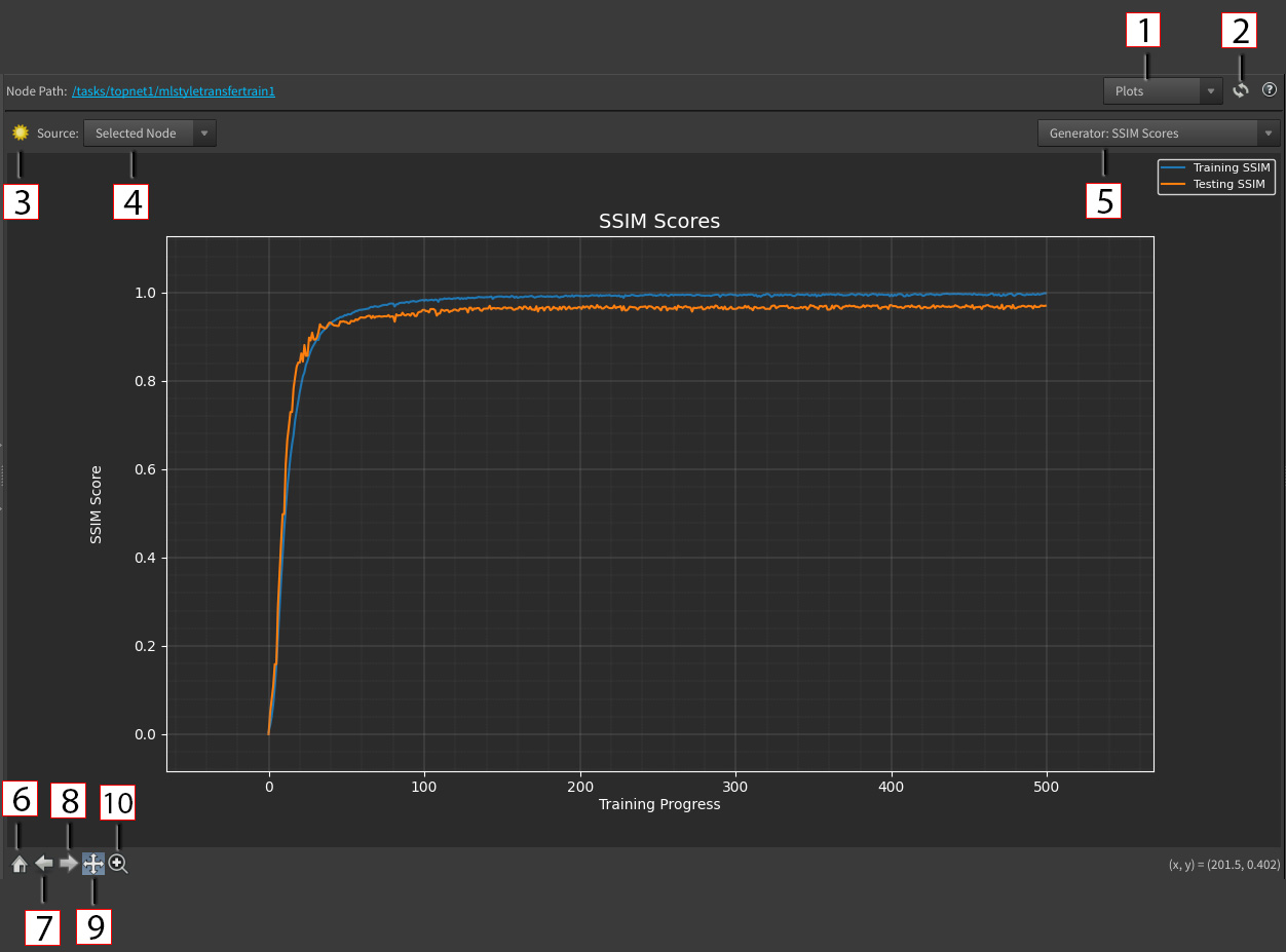
1 - Panel Mode dropdown: Determines the panel display. Options are Plot and Test Results.

Plot: View training metrics and trends over time using interactive plots. Useful for visualizing things like loss curves and evaluation scores.
Test Results: View image outputs generated by the model during testing.

2 - Refresh: Refreshes the panel.
3 - Light Mode: Toggle plot between light and dark mode.
4 - Source Dropdown: Options are Selected Node and Custom File.

Selected Node: The source of the plot is based on the CSV file provided by the node’s ml_description function.
Custom File: The source of the plot is based on a user uploaded CSV file, independent of the selected node.

5 - Plot Dropdown: The specific plot that is being displayed. The convention is always the model name followed by the plot title.

For example, if the node has a Generator and Discriminator model, the Generator has a Loss and Score plot, and the Discriminator has a Score plot, then the dropdown options would be:
- Generator: Loss
- Generator: Score
- Discriminator: Score

6 - Home: Reset original plot view.
7 - Back: Back to previous plot view.
8 - Forward: Forward to next plot view.
9 - Pan Mode: Select drag with LMB to move the view of the plot without changing the zoom level. This mode is on by default.
10 - Zoom Mode: Select drag with LMB to draw a rectangle on the plot. The view will zoom into that area.

You can also zoom using your scroll wheel and does not require zoom mode.

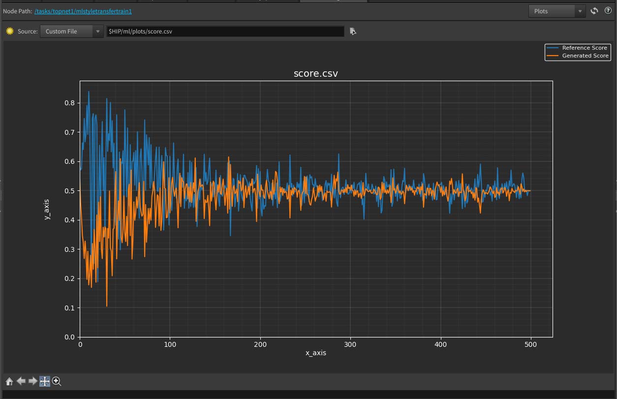
Plotting with custom file path ¶

By default, the data plotted will be based on the selected ML node. However, you can also view plots from a custom CSV file by selecting Custom File in the source dropdown. You can either upload a file or type in the path in the text field beside the source dropdown. Houdini formatted paths are acceptable.

Example plot generated from a custom user-uploaded CSV file showing evaluation scores over time

Viewing test results ¶

The test results panel allows you to view your model’s output images during testing. Both the displayed images and their categories (e.g input, reference, generated) vary depending on the node configuration, model, test number, and epoch.

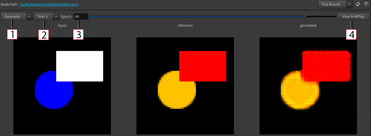
1 - Model name dropdown: The ML model’s images to display.

For example, if the node has a Generator and Discriminator model, then the dropdown options will be
- Generator
- Discriminator

2 - Test number dropdown: The test’s images to display.

The number of items in this dropdown is based on the test size per epoch.
For example, if the test size is 2, then there are 2 sets of test images per epoch, so the dropdown options will be
- Test: 0
- Test: 1

3 - Epoch Text Field: The epoch’s images to display. Can be modified by editing text field or dragging slider using arrow keys, mouse drag, or mouse scroll.
4 - View in Mplay: View the images in an external image/animation viewer.