The following chapters guide you through the creation of a basic Vellum fluid simulation using all three methods. The scene uses a sphere to source Vellum fluid particles and create a drop. The drop is then attracted by gravity and collides with a glass. Each method should create the same results.

Download and open the scene file with the sphere and glass objects as a starting point.

The sphere is located inside the source_geo node, the glass inside glass_geo. Both containers are Geometry OBJs. Note that this setup isn’t a real world scenario. For demonstration purposes, scene scale is very big. When you open the file, you should see this:

The idea behind Houdini’s shelf tool is to provide fast access to preconfigured setups. You don’t have to think about different types of networks, connections or data exchange between DOP and SOP networks. Anyway, shelf tools don’t save you from configuring your simulation, adjusting solver settings, and so on. What you get from these tools is a fundamental setup you can start working with.

The shelf method is already a DOP version and you can use the shelf setup as a template for examining and recreating the networks manually.

Start with the source geometry and the Vellum Solver DOP.

1. Select the source_geo Geometry node. The Sphere SOP inside acts as the source object for the particles.

2. Open the Vellum shelf and click Vellum Grains. After a few moments Houdini dives into a newly created AutoDopNetwork DOP Network node. The sphere is no longer visible, but now you can see some particles instead.

3. In the Network Editor, press L for a clean node layout.

4. Click the vellumsolver1 node to see its parameters.

5. For fluids, the default Substeps value is 5. Enter a value of 10 to get higher precision.

6. A Constraint Iterations value of 20 is sufficient for fluids.

7. Smoothing Iterations are not required here and should be set to 0.

The shelf tool created the AutoDopNetwork and a grains_vellum Geometry node on obj level. The latter node is described later. Now the fluid properties are adjusted.

1. On obj level, double click source_geo to dive into the node.

2. Turn on the GEO node’s blue Display/Render flag to see the particles.

3. Click the grain_constraints node. This node is a Vellum Configure Grain SOP and is currently configured as a grain source.

4. Change Type to Fluid.

5. With Particle Size you can change the number of particles. For this scene, use a value of 0.01.

6. Change Packing Density to 1.5 for a better particle representation of the source object.

7. Open the Physical Attributes sub-pane.

8. Set Mass to Calculate Uniform. This action unlocks the Density parameter. The default value of 1000 describes water and can be kept.

The glass should act as a collision object and interact with the particles. To establish this connection, you can use another shelf tool.

1. Go back to obj level and select the glass_geo node.

2. Open the Collisions shelf and choose Static Object.

3. Dive into AutoDopNetwork again, and press L to reorganize the nodes. You can now see a new branch in the network, introducing glass_geo as a collision object.

The scene is now ready to simulate, but you can further explore all networks to become more familiar with the nodes. If you want to cache the result, go back to obj level and dive into grains_vellum. The vellum_io node provides two options for saving the simulation to disk.

• Save to Disk opens a progress bar and Houdini’s UI is locked during simulation.

• Save to Disk in Background asks if you want to save the project. During simulation, the UI remains responsive.

• For simulating without saving, press the button.

In SOP-based setups you can create the entire network within in a single Geometry OBJ node. You don’t have to separate networks and exchange data. However, with complex networks it makes sense to keep things separated and store different parts of the scene in different Geometry OBJs. Create a new scene and reload the file with the base setup. Start with the source object to create the fluid particles.

1. On obj level, double click source_geo to dive into the node.

2. Press ⇥ Tab to open the TAB menu, and enter config fluid. Choose the only result Vellum Configure Fluid. You can see that this node is a Vellum Configure Grain SOP, but Type is set to Fluid already.

3. Set Particle Size to 0.01 to get more particles.

4. The Packing Density parameter is 1.5 for a better particle representation of the source object.

5. Connect the sphere1 node’s output with the first input of vellumfluid1.

6. Turn on the vellumfluid1 node’s blue Display/Render flag to see the particles.

The next stop is the Vellum Solver SOP where you determine simulation settings.

1. Press ⇥ Tab and enter solver. From the list, choose Vellum Solver.

2. Set the solver’s Substeps to 10. This is the recommended value for Vellum fluids.

3. Decrease Constraint Iterations to 20 to make particle constraints less stiff.

4. Smoothing Iterations are not required for fluids and you can set them to 0.

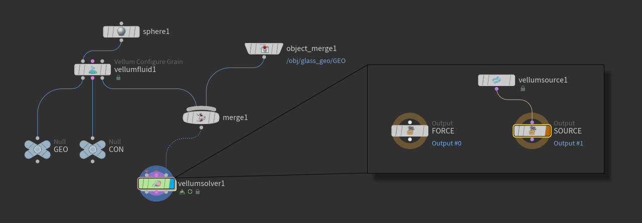
In many cases the next step is to connect the outputs of vellumfluid1 with the inputs of vellumsolver1. For this setup, we use a different approach.

1. Press ⇥ Tab. Enter null and create two Null SOP nodes.

2. Rename one Null to GEO, the other to CON.

3. Connect the GEO node’s input with the first output of vellumfluid1 - the Geometry output.

4. Connect the CON node’s input with the second output of vellumfluid1 - the Constraints output.

5. Link the third output of vellumfluid1 with the third input of vellumsolver1.

If you went through the Shelf tool and DOP workflows chapter, you might came across a Vellum Source DOP node. There, the node establishes a connection between particles, constraints, and the solver. Here, the Vellum Source provides fast access to the Emission Type parameter. With this parameter you can choose, whether you want to source particle once, per frame or per substep. With direct connections between vellumfluid1 and vellumsolver1 you'd have to unlock the solver and dive deep into its network to access Emission Type.

1. Double click vellumsolver1 to dive into the node.

2. Press ⇥ Tab to add a Vellum Source DOP.

3. Connect the vellumsource1 node’s output with the input of SOURCE.

4. Select the source node to access its parameters.

5. For Source ▸ SOP Path enter /obj/source_geo/GEO.

6. For Source ▸ Constraint SOP Path enter /obj/source_geo/CON.

7. Return to obj level.

Now connect the glass as a collision object for the particles. The shelf tools workflow uses a static solver. Here you take a shortcut through a direct connection.

1. Press ⇥ Tab to add a Merge SOP and an Object Merge SOP node.

2. Place merge1 between the third output of vellumfluid1 and the third input of vellumsolver1.

3. Link the object_merge1 node’s output to merge1.

4. Select object_merge1 and look for the Object 1 parameter. There, enter /obj/glass_geo/GEO to import the glass’s geometry from glass_geo. Once the connection is active you can see a blue wireframe representation of the glass.

Collision objects can be directly connected to the Vellum Solver’s fouth input (Collision Geoemtry). Vellum fluids use a geometric approach and therefore, objects must be polygons. If necessary, add a Convert SOP with Convert To set to Polygon.

It’s also possible to add collision geometry to the Vellum Configure Grain SOPs third input (Collisions). Once connected, objects appear as a blue grid in the viewport. If you want to hide this grid, go to the Vellum Solver and turn off Visualize ▸ Show Collision.

Another way to connect collision geometry is through a shelf tool. Note that this method is only available for DOP setups, and the Vellum fluids network has to exist before you execute the tool. Select the object you want to use. Then, go to the Collisions shelf and choose, as already mentioned earlier, the Static Object tool.

The shelf tool’s network comes ready to use with a Vellum I/O SOP node to cache the simulation results to disk. In manually created networks this node has to be added. For simulating without saving, press the button.

1. Add a Vellum I/O SOP and connect its inputs to the outputs of vellumsolver1.

2. Press Save to Disk (locked UI) or Save to Disk in Background (responsive UI) to cache the simulation data.