| On this page |
By default, Vellum constraint and solver nodes don’t provide dedicated parameters to determine an exact emission direction. Particles only follow the solver’s built-in forces gravity and, if active, wind. Let’s say, for example, you want to emit particles along a source object’s normals or make the fluid move upwards in a 60° angle. Such tasks require a custom function to set the particles' initial direction at creation time.
If you want to change the particles' trajectories, you can add POP forces. Houdini provides preconfigured POP nodes, but it’s also possible to assemble custom forces through a ![]() POP VOP DOP. One of the most common forces is
POP VOP DOP. One of the most common forces is ![]() POP Drag DOP. This force mimics air friction and helps to decelerate fast moving fluids and keep the particles together. Another very useful node is the
POP Drag DOP. This force mimics air friction and helps to decelerate fast moving fluids and keep the particles together. Another very useful node is the ![]() POP Attract DOP. Here you can direct particles towards a goal position. Typical examples for POP VOP forces are Curl Noise VOP or
POP Attract DOP. Here you can direct particles towards a goal position. Typical examples for POP VOP forces are Curl Noise VOP or ![]() Turbulent Noise VOP to randomly displace particles and create interesting structures.
Turbulent Noise VOP to randomly displace particles and create interesting structures.
Initial direction 
The introduction already mentioned two common problems: it’s not obvious how to emit particles along an object’s normals or specify a certain angle for emission. In both cases, speed is the key. The task is to modify the particles' velocity, so they move in a certain direction. In the image below you can see the normals of a basic ![]() Sphere SOP. The idea is to use the normals as a “guide” for the particles by converting those normals into velocity. Normals and velocity consist of XYZ components and together they form a vector. In the example setup below, particles are scattered across a sphere’s surface and then accelerated along the normals.
Sphere SOP. The idea is to use the normals as a “guide” for the particles by converting those normals into velocity. Normals and velocity consist of XYZ components and together they form a vector. In the example setup below, particles are scattered across a sphere’s surface and then accelerated along the normals.
Basic fluid setup 
Note
The example scene is SOP-based. If you're looking for a DOP network or a shelf tool method, please visit the Vellum fluids setups page. You can find detailed information there on how to use the different methods for setting up Vellum fluids.
-
On obj level, press ⇥ Tab to invoke the TAB menu. From there create a
 Geometry OBJ and double click it to dive into the node.
 -
Create a
 Sphere SOP.
 -
Set Uniform Scale to
0.5. -
Increase Rows to
52and Columns to96to get a smoother surface. -
Click the Display Normals
 icon to make the normals visible. If the normals are too long, move the mouse cursor over the viewport and press D. This hotkey opens the Display Options. Click the Guides tab and set Scale Normal to
 0.05. -
Add a
 Scatter SOP and connect its input with the Sphere SOP’s output.
 -
In the Scatter node, increase Force Total Count to
10000to get enough particles.

Now, create the Vellum fluid network.
-
Add a
 Vellum Configure Fluid SOP node.
 -
Connect the first input with the Sphere’s output to transfer the particles.
-
Turn off Create Points from Volume to cover the surface.
-
Set Particle Size to
0.005or smaller to see the individual fluid particles. -
Add two
 Null SOPs and connect them to the first (Geometry) and second (Constraints) output of the Vellum Configure.
 -
Rename the first output’s Null to
GEO(geometry), the second toCON(constraints). -
Add a
 Vellum Solver SOP.
 -
Connect the Vellum Configure node’s third output to the third input (Collision Geometry) of the solver.
Note, that the other two inputs remain empty, although they're mandatory. The connection will be established through another node inside the solver. You might notice that all normals point in negative Z direction. What you're seeing now are the particle normals.

-
Double click the Vellum Solver to dive into it.
-
From the TAB menu, add a
 Vellum Source DOP.
 -
Connect it to the
SOURCE Output DOP.
 -
Go to SOP Path and type
/obj/geo1/GEO. -
For Constraint SOP Path, enter
/obj/geo1/CON. Now, geometry and constraints are connected to the solver. The reason for this detour is that you now have access to the Emission Type parameter. -
From the Emission Type dropdown choose Each Substep.
-
Return to geo1 level and click the Vellum Solver to access its parameters.
-
In the Solver tab, increase Substeps to
5- the standard value for fluids. -
Decrease Constraint Iterations to
20to make the fluid less rigid. -
Fluids don’t need Smoothing Iterations and you can set them to
0. -
Open the Forces tab and change Gravity to
0,0,0.
Introducing the normals 
When you simulate, you can see that only a few particles randomly move. To make the particles follow the Sphere’s normals, two more nodes are required.
-
Return to geo1 level and open the TAB menu. Add two
 Point Wrangle SOPs.
 -
Place the first Wrangle between Sphere and Scatter to connect it.
-
In the VEXpression field, enter
@N = @N;(including the trailing semicolon). This VEXpression takes the Sphere’s normals and stores them in a new@Nvariable.@Nis a standard geometry attribute like@Pfor position. Houdini recognizes standard variables and their data types. Normals, for example, are vectors. Vectors can be split into their components using@N.x,@N.yand@N.z. This is useful if, for example, you only want to use the normals' Y values, while replacing X and Z through your own formulas or fixed values. -
Turn on the Vellum Configure Grain node’s blue Display/Render flag.
You can now see the particles' normals pointing away from the sphere. The object’s normals are transferred to the particles.

Velocity from normals 
In this step, the normals are used to define a velocity. Since you don’t know how fast the particles will be at creation time, it’s a good idea to introduce a factor to control their speed.
-
Place the second Point Wrangle between Scatter and Vellum Configure to connect it.
-
In the VEXpression field, enter
v@v = set(normalize(@N) * chf("speed_multiplier"));. Again, don’t forget the semicolon!
The expression introduces a velocity vector v@v. @v is another standard attribute like @N, so the name must not be changed. The set command sets the velocity vector. You don’t have to define the XYZ vector components manually, because @N is already a vector. The normalize function recalculates the normals to values between 0 and 1. This process can be seen as a standardization and returns predictable results. Finally, a custom parameter speed_multiplier is introduced. With this value it’s possible to scale the particles' initial speed.
-
Click the
 icon to expose the custom Speed Multiplier parameter. Enter a value of
 0.2. -
Turn on the Vellum Solver’s Display/Render flag and click
 to simulate.
The particles follow the Sphere’s normals and you can make them slower or faster with the custom Speed Multiplier parameter.
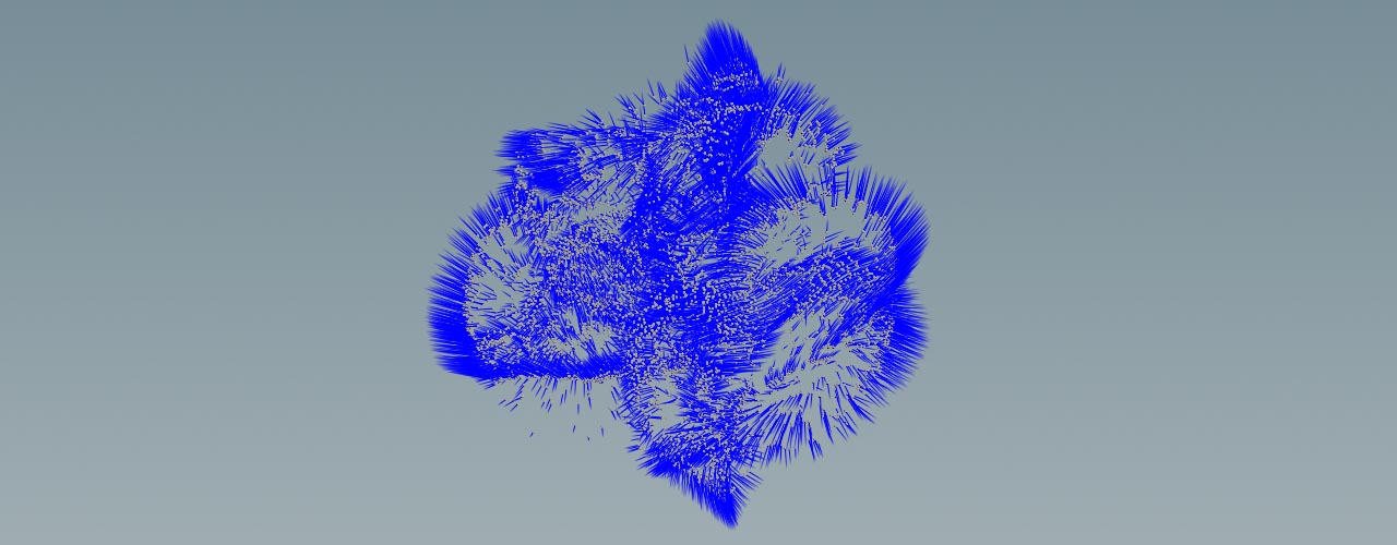
Normals are perpendicular to their associated polygons, but you can randomize the normals through another VEXpression. There are endless possibilities and you can combine various VEXpression functions to get interesting results.
-
Select the first Attribute Wrangle. In the VEXpression field, add another line and enter
@N = curlnoise(@N);to create a curly normal field. Thecurlnoisefunction looks good with spherical objects as shown below.
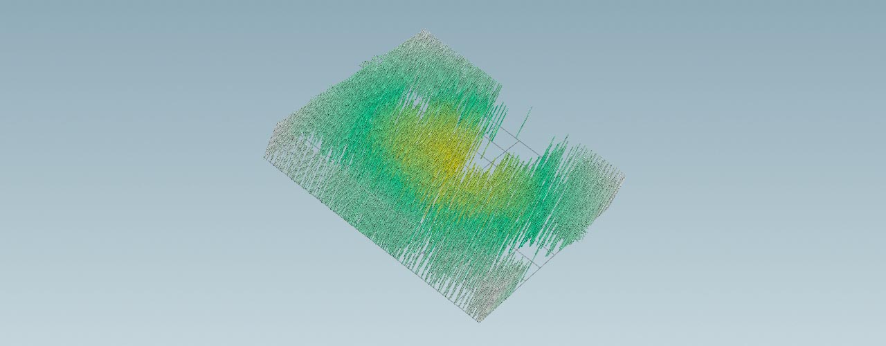
Custom emission direction 
The normal method can also be used for 2D emitters like grids. This way it’s possible to shoot particles into a certain direction just by rotating the grid. For a smooth particle stream, dive into the Vellum Solver and change the vellumsource1 node’s Emission Type to Each Substep. To invert emission direction, make the object normals negative: v@normals = -@N;. The grid’s Rotate values in the image below are 45,0,30.
Another way is to define a custom initial velocity. Normals aren’t required here and you can therefore delete the two Wrangles if not already done.
-
Add a new Point Wrangle SOP and place it between Scatter and Vellum Configure.
-
If you have a Grid SOP as particle source, replace it through a small Sphere SOP.
-
Velocity is a vector, consisting of XYZ components. For a complete vector, you have to define three values. In the VEXpression field, start with
v@v = set();. This expression tells Houdini to set an initial velocity. The actual XYZ values are written in the brackets. -
You can use any valid function. The function can be static, time-dependent, or a combination of both methods. A complete velocity vector could look like this expression:
v@v = chf("speed_multiplier")*set(sin(@Frame/4),0,cos(@Frame/4));.
Applying forces 
The first decision is whether you want to work with DOP or SOP networks. Both network types accept POP forces to drive the particles, but there’s a difference where to add those forces.
-
In the Vellum Solver SOP’s Force tab you can find Gravity and Wind parameters. In SOP networks, double click the Vellum Solver to dive into it. Inside the node you can see an
Output DOP named FORCE. This is where new forces are linked to. -
The Vellum Solver DOP lacks a Force tab and even standard gravity has to be introduced through a separate downstream node. This applies to all forces in DOP networks.
This example explains how to make particles follow a spiral and can be seen as blueprint for the usage of force in Vellum. The scene uses a SOP setup. In DOP networks, e.g. created through the ![]()
![]() Vellum Grain shelf tool, forces are added inside the
Vellum Grain shelf tool, forces are added inside the ![]() AutoDopNetwork DOP before or after the solver.
AutoDopNetwork DOP before or after the solver.
Particle path 
The fluid’s path is created from a deformed spiral.
-
On obj level, press ⇥ Tab to invoke the TAB menu and create a Geometry OBJ. Double click the node to dive into it.
-
Create a
 Helix SOP.
 -
Change Height to
5. -
Turns is
1.8. This is the number of Turns over the curve’s Height. -
In the Radius section, change Start Radius to
0.25to make the spiral thinner. -
Go to Construction and shift the spiral’s start point by increasing Start Angle to
120degrees. -
Divisions per turn should be
100to get a smoother curve.
The spiral is deformed to get more turbulence.
-
Add an
 Attribute Noise SOP and connect its input to the upstream Spiral node.
 -
Under Attribute Names, delete
Cdand enterPforposition. -
Change Amplitude to
0.3to smooth the spiral and avoid extreme displacement. -
You can create more structure by decreasing Noise Pattern to
0.7.
Transform the spiral to set its start to the scene’s origin.
-
Add a
 Transform SOP. Connect the input with the Attribute Noise node’s output.
 -
Set Translate to
-0.1,0.02,0. -
For Rotate use
0,45,-90degrees to tilt the spiral and align it with the X axis.
Vellum fluid network 
Note
The Vellum fluid network has been discussed several times, e.g. in the Basic fluid setup chapter above. For this scene, a reduced workflow description describes the most important step.
-
Create a Sphere SOP and set its Uniform Scale to
0.2. Check, if the spiral’s starting point is inside the Sphere. -
Add a Vellum Configure Fluid SOP and connect its first input with the Sphere’s output.
-
Set Particle Size to
0.007to get enough particles. -
Expand the Physical Attributes subpane, turn on Surface Tension and enter a value of
25. -
Add two Null SOPs and rename them to
GEOandCON. -
Connect
GEOto the Vellum Configure node’s first output,CONto its second output.
In the next step, configure the solver.
-
Lay down a Vellum Solver SOP. Connect the third input with the third output of the Vellum Configure SOP.
-
Change Solver ▸ Time Scale to
0.25to make the simulation 4× slower. -
For the following three parameters (Time Steps, etc.) use the standard values for fluids:
5,20, and0. -
Open the Forces tab and set Gravity to
0,0,0. -
Double click the solver to dive into it.
-
Add a
Vellum Source DOP and connect it with the SOURCEnode. -
For SOP Path, enter
/obj/geo1/GEO. -
For Constraint SOP Path, enter
/obj/geo1/CON. Particles and constraints are now connected to the solver. -
From the Emission Type dropdown choose Each Substep.
-
Go to Activation and type the following expression:
$FF<50. When the current frame is smaller than 50, particles are sourced. Starting with frame 50 the source is inactive.
Forces 
The particles should follow the spiral and wind around it. There should be drops, but also a main body of fluid with enough turbulence to create an interesting look. Start with the curve force.
-
Inside the Vellum Solver, add a
 POP Curve Force DOP and connect it to the
 FORCEnode. -
For SOP Path, enter
/obj/geo1/transform1. This is the last node of the spiral’s network. -
Max Influence Radius is
0.4. When you change the value you can see that the red tube becomes thinner. The tube marks the area, where particles are influenced by the curve force. -
Follow Scale is
4. This force makes the particles move along the curve. -
Suction Scale is
12to attract the fluid towards the curve. -
An Orbit Scale of
3creates a rotational force around the curve.
It can be tricky to balance forces: when you increase one force, you normally have to decrease another parameter to avoid overshooting effects. If the particles are too fast, it’s a good idea to decelerate them.
-
Add a
 POP Drag DOP and place it between curve force and
 FORCE. -
Air resistance slows down the particles. Here, enter a value of
0.62.
When you simulate, the fluid follows the spiral, but there’s hardly any turbulence and everything looks smooth. To get more randomness, do the following.
-
Add a
 POP Force DOP and place it between curve force and drag force.
 -
Under Noise ▸ Amplitude, enter
17. The noise field rips the fluid apart and creates droplets.
Start the final simulation and watch the fluid winding around the curve. There are thinner and thicker areas, the particles are decelerated at the spiral’s turns and you see drops. After approximately 120 frames, the first particles start to leave the spiral. You can limit the simulation to 150 frames.