In Houdini and Mantra, Primitives all have an implicit parametric space, sometimes called primitive UVs, for referring to positions on their surfaces, or other interpolations of Geometry attributes on their points or vertices.

Coordinates in these spaces can be output by the Ray or Scatter nodes, or the intersect, intersect_all, xyzdist, uvintersect, or uvdist VEX functions. These coordinates can then be used for interpolation within primitives, for example, if they're deforming over time, by the Attribute Interpolate node or the primuv VEX functions.

There are many primitive types in Houdini, each with special parametric spaces:

• Polygons: Triangles and Quads, n-gons, Polygon Curves, Degenerate

• Polygon Soups

• Tetrahedra

• Volumes

• VDBs

• Packed Primitives

• Bezier/NURBS/Bilinear Surfaces

• Bezier/NURBS Curves

• Quadrics: Spheres, Tubes, Circles

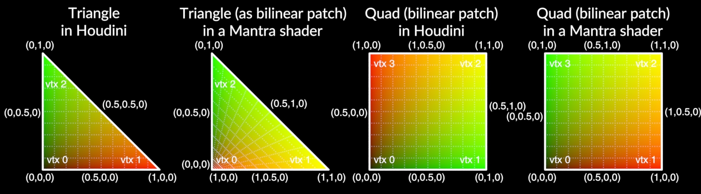
Triangle parametric spaces in Houdini have vertex 0 at the origin, (0,0), vertex 1 at the u axis unit, (1,0), and vertex 2 at the v axis unit, (0,1). u and v are equivalent to two “ barycentric coordinates ” of the triangle, namely the barycentric coordinates associated with vertex 1 and vertex 2. The barycentric coordinate associated with vertex 0 is 1-u-v. These give the 3 linear interpolation weights for the 3 vertices, e.g. P(u,v) = P0*(1-u-v) + P1*u + P2*v. Half of the uv unit square is unoccupied, though some cases may mirror the other half onto the first half if provided coordinates out of range.

Quads are treated as bilinear patches in Houdini, to smoothly, consistently handle cases where the 4 vertices are not all in the same plane (non-planar), at the expense of that quads are quadratic surfaces, instead of flat surfaces like triangles. Quad parametric spaces also have vertex 0 at the origin, however, vertex 1 is instead at the v axis unit, (0,1), and vertex 3 is at the u axis unit, (1,0); vertex 2 is at (1,1). Bilinear interpolation is done in a manner within roundoff error of P(u,v) = P0*(1-u)*(1-v) + P1*(1-u)*v + P2*u*v + P3*u*(1-v).

Note that non-convex quads will usually still be treated as bilinear patches, which will self-overlap in these cases. This is sometimes unwanted, so if you need non-convex quads to be triangulated, you can use the Divide geometry node with Convex Polygons enabled, and Maximum Edges set as needed, e.g. 4 if you want to keep convex quads as quads. Bowtie quads are more difficult to split well if the bilinear interpretation is not acceptable, but can be fixed with a combination of options on the Triangulate 2D.

In a Mantra shader, the implicit u and v coordinates of a quad are swapped relative to those in Houdini, which doesn’t frequently cause problems, but may be confusing if working directly with implicit uv’s in a shader. For triangles in Mantra, the implicit uv coordinates of a triangle will be those of a quad (bilinear patch) with vertex 0 duplicated. This results in interpolation of attributes on triangles that’s equivalent to the interpolation in Houdini, even though one is interpolated bilinearly and the other is interpolated barycentrically.

The triangles and quads in the diagram all have normals pointing into the screen, so these are showing the back faces. The normal direction is “left-handed” relative to the winding order. Many other 3D geometry programs use “right-handed” normals, so you may need to use a Reverse node to reverse the winding order of polygons when importing from another software package.

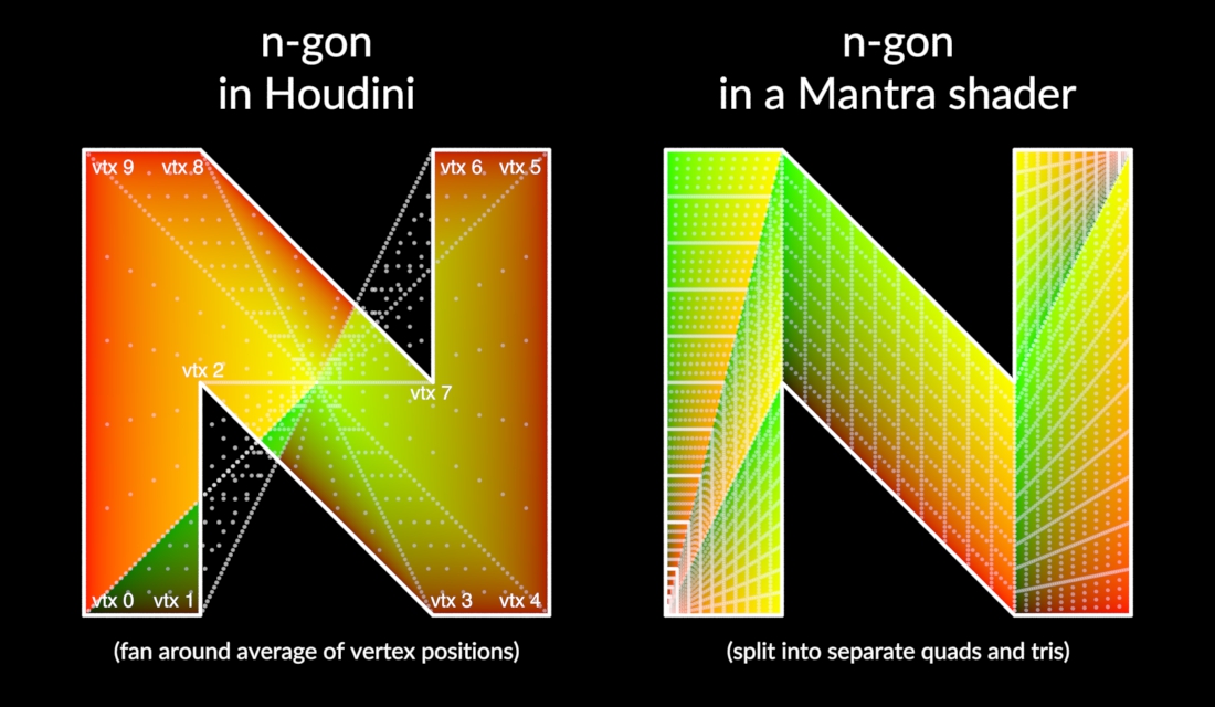
Polygons with 5 or more sides are often referred to as “n-gons”, to distinguish that they need to be handled differently from triangles or quads.

In order to have at least one implicit uvw coordinate corresponding with each point in a non-convex n-gon, Houdini implicitly covers the space with a triangle fan around the average of all of the vertices. Each edge contributes 1/n to u, where n is the number of vertices. v is 0 on an edge, and approaches 1 linearly toward the center. The boundary parameterization is equivalent to that of a polygon curve if it had an extra vertex wrapping it back around to vertex 0.

However, because there are polygons that are not “ star-shaped ” or that do not have the center in their kernels, there can be both points outside the polygon that have parametric coordinates in the unit square, and points inside the polygon that have multiple parametric coordinates, (possibly even multiple positions if the polygon is non-planar). A single implicit uvw coordinate still always represents a single position. This usually doesn’t cause problems if the coordinates are generated by nodes or VEX functions that output primitive uvw coordinates, but may be confusing when trying to separately generate or interpret them. It does, however, mean that for polygons with many sides, the time required to determine the coordinate or interpolate the polygon from one takes time proportional to the number of sides, so can be slow for polygons with hundreds or thousands of sides.

Mantra always splits polygons with 5 or more sides into triangles and quads, with a similar method to the one used by the Divide geometry node with Maximum Edges set to 4. This avoids some issues of the coordinate system used in Houdini, but at the expense of multiple positions having the same parametric coordinate and instability. Slight changes in the positions of the vertices can result in the polygon being divided differently, so when rendering deforming geometry that may have n-gons, be sure to divide the rest geometry before deforming so that there are no n-gons and the topology doesn’t change from frame to frame. This will avoid any popping in the renders that would have come from the n-gon splitting changing.

The n-gon in the diagram has normals pointing into the screen, so this is showing the back face. The normal direction is “left-handed” relative to the winding order, just as with triangles and quads. Many other 3D geometry programs use “right-handed” normals, so you may need to use a Reverse node to reverse the winding order of polygons when importing from another software package.

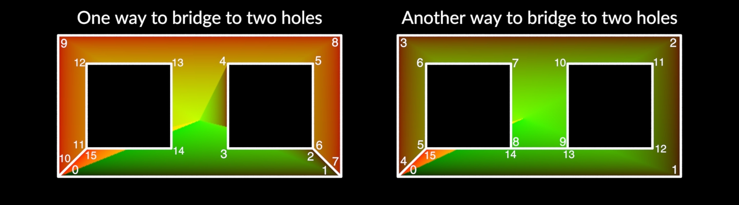
Polygons in Houdini can also have what are known as “bridges”, which are edges a polygon shares with itself, to be able to construct “holes”. Bridges require having multiple vertices of the polygon visit the same points more than once, which isn’t allowed in some other software packages, so when exporting to other software, you may have to divide polygons that have bridges, and when importing from software that has explicitly separate hole polygons, you may have to apply a Hole node to correctly create the bridges to holes.

There are many ways to create bridges to holes, especially if there are multiple holes, since a hole can bridge to another hole, as shown in the diagram. The one primary requirement of bridges is that they are not allowed to cross an edge of the polygon, including other bridge edges and edges of the holes.

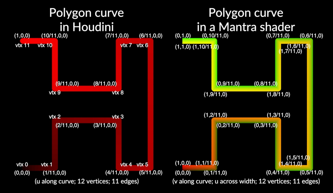
In Houdini, polygon curves have a parametric u coordinate that starts with 0 at vertex 0 and ends with 1 at vertex n-1, each edge adding 1/(n-1) to u, where n is the number of vertices in the curve. v and w are both zero.

In a Mantra shader, however, v goes from 0 to 1 along the curve, just like u does in Houdini, with each edge contributing 1/(n-1). Curves also have width in Mantra, and u goes from 0 to 1 along the width of the curve.

It is possible in Houdini to construct polygons that don’t have enough vertices, so are considered degenerate, but are not automatically deleted. Closed polygons with 0, 1, or 2 vertices are degenerate, and open polygons (polygon curves) with 0 or 1 vertices are degenerate. Although it’s often not meaningful to compute something for such primitives, it’s important to not crash, loop infinitely, or use infeasible amounts of memory when nodes or assets are provided such polygons in their input.

The parametric space of a polygon with zero vertices is ill-defined. The parametric space of a polygon with 1 vertex should have that vertex fill the entire space, or put in the reverse sense, all parametric coordinates map onto that vertex. A closed polygon with 1 vertex is sometimes treated as having 1 edge from its vertex back to itself, to maintain that the number of edges is equal to the number of vertices, though other times it is treated as having no edges. A closed polygon with 2 vertices is sometimes treated as a polygon curve with 2 vertices, though it is sometimes treated as having two of the same edge.

Polygon soups represent multiple faces in a single primitive. Each face has implicit u and v coordinates equivalent to the corresponding coordinates of an equivalent closed polygon primitive.

The w coordinate is used to indicate which face in the soup is referenced. If the face number within the soup is 16,777,216 (i.e. 2^24) or smaller, w is just the floating-point value of the face number. For faces beyond that (up to 1.9 billion faces), w is guaranteed to be a unique, positive, non-infinite, non-NaN, non-denormal floating-point number, so that it will be preserved if multiplying by 1 or adding 0. The w coordinate can be generated from the face number using the pack_inttosafefloat VEX function, and the face number can be retrieved from a w coordinate using the unpack_intfromsafefloat VEX function. In the HDK, these correspond with the functions UTpackIntToSafeFloat and UTunpackIntFromSafeFloat in UT_SafeFloat.h .

Tetrahedra (tets) in Houdini are sometimes considered solid, e.g. when using the xyzdist VEX function or the Minimum Distance option in the Ray node. This is useful for determining the parametric coordinates of points of a point cloud embedded in a tetrahedral mesh. However, sometimes only the unshared faces, the surface of a tetrahedral mesh, are considered, e.g. when using the intersect function or the Project Rays option in the Ray node. The boundary of the tetrahedral mesh, transition into or out of it, is more likely to be the desired result in these cases.

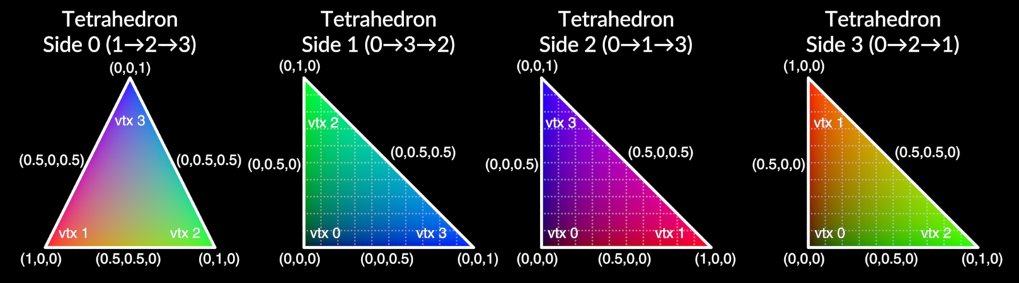
In both situations, the parameteric uvw coordinates are reported the same way. Similar to triangles, vertex 0 is at the origin, (0,0,0), vertex 1 at the u axis unit, (1,0,0), vertex 2 at the v axis unit, (0,1,0), and vertex 3 at the w axis unit, (0,0,1). Also similar to triangles, u, v, and w are equivalent to the barycentric coordinates associated with vertex 1, vertex 2, and vertex 3. The barycentric coordinate associated with vertex 0 is 1-u-v-w. These give the 4 linear interpolation weights for the 4 vertices, e.g. P(u,v,w) = P0*(1-u-v-w) + P1*u + P2*v + P3*w. 5/6 of the uvw unit cube is unoccupied, though some cases may mirror coordinates into the valid region if provided coordinates out of range.

The triangular faces in the diagram all have normals pointing into the screen, so these are showing the back faces. The normal direction is “left-handed” relative to the winding order, as with polygon primitives. Tetrahedra have the additional consideration that they can be inverted, i.e. having negative signed volume. If the normals of a tetrahedron’s faces point inward, (toward the opposite vertex), it is inverted; if they point outward, it is not inverted. Note that if you assign the implicit uvw coordinates corresponding with each vertex to the point positions, the tetrahedron will be inverted.

All tetrahedra are assumed to have 4 vertices. If one is constructed in the HDK with a different number of vertices, code may crash or produce nonsensical results. The addprim and addvertex VEX functions will not allow construction of one with a different number of vertices.

Volumes only have one vertex, so there is only interpolation of P and voxel values. A single volume primitive in Houdini only represents a single 32-bit floating-point value in each voxel. Multiple volume primitives can be logically grouped into an effective vector volume using a name primitive string attribute, using names like “Cd.x”, “Cd.y”, and “Cd.z”. Volumes that have only one voxel in one of the parametric directions, 2D volumes, can be treated as flat images in various places in Houdini. Volume primitives can be 2D or 3D “fog volumes”, 3D “signed distance fields” (SDFs), or 2D “heightfields”.

For computing positions, parametric coordinates for a volume in the range (0,0,0) to (1,1,1) are first converted to the range (-1,-1,-1) to (1,1,1), and then any taper (for frustum volumes), the 3×3 local transform, and the translation from P are applied. The inverse is done (in the reverse order) to compute parametric coordinates for a position. For 2D heightfield volumes, the value of the volume evaluated at the parametric coordinates for the axes that have more than 1 voxel in them, is used as the displacement from the center plane along that axis.

Voxel data in volume primitives are treated as cell-centered. Between voxel centers, data are interpolated trilinearly . The 0 and 1 parametric values correspond with the beginning of the first voxel and the end of the last voxel in some parametric axis, respectively. These coordinates are not between voxel centers, though, being on the boundary, so are handled like out-of-bounds values, using either the “constant”, “repeat”, “streak”, or “sdf” border type, (which can be seen in the volumebordertype primitive intrinsic). “constant” indicates to use a constant value, (in the volumebordervalue primitive intrinsic), “repeat” indicates to wrap around the voxel grid, so that coordinates are always between voxel centers, and “streak” indicates to use the value that would be evaluated if the coordinate were snapped to the closest boundary between voxel centers. “sdf” indicates to add the distance to the closest boundary voxel data when evaluating, and also in some situations, treat the volume as the surface implied by places in the voxel data that cross between positive and negative. The voxel data are intended to be signed distances to the implicit surface.

Voxel data in volume primitives are stored in 16×16×16 tiles, or smaller for end tiles in any axis that has a resolution that is not a multiple of 16. A tile that contains only a constant value for all of its voxels can be represented by that single value, instead of a full grid of its data. This allows more efficient representation of sparse volume data.

VDBs are an open standard volume representation optimized for very sparse volume data, usually only having bottom-level voxel data in a “narrow band”, using a 4-level tree of tiles that can be constant at any level. The top level can be an arbitrary resolution, but the other levels are a fixed power-of-two resolution in each tile, down to voxels at the bottom. Unlike most other primitive types, the parametric space of a VDB is not limited to the range (0,0,0) to (1,1,1). The space is identical to the bottom level voxel index space, and voxel indices can be negative, depending on the shift of the top level grid. This allows adding of new voxel data anywhere (up to roundoff error considerations), without changing the parametric coordinates of existing data. The transform of the VDB grid, (including any frustum transform), transforms directly from voxel index space to physical space.

VDBs most often represent “signed distance fields” (SDFs), also referred to as a “level set”. However, often only the narrow band has correct signed distances to the implied surface, whereas the constant tile data values outside of the narrow band may only have the correct sign, not an actual distance. Some VDBs instead represent “fog volumes”, where the values represent densities or other values. Outside of the range of occupied tiles, there is a “background value” of any given VDB.

Like volume primitives, VDBs only have one vertex, so there is only interpolation of P and voxel values. Unlike volume primitives, a voxel’s data in a VDB can be a 32-bit or 64-bit floating-point number, a 32-bit integer, a boolean, a vector of three 32-bit or 64-bit floating-point numbers, or a vector of three 32-bit integers. From the HDK, VDB grids that are created directly, instead of part of a primitive, they can have other data types.