The basic setup makes you familiar with the most fundamental requirements, workflows and settings. Start with changing the active desktop to Solaris. You can choose this desktop from the first dropdown in Houdini’s main menu.

The network, described below, contains the recommended layout.

Render environment setup ¶

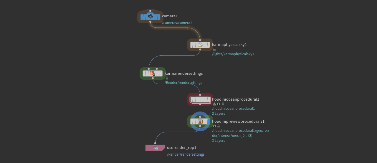
The render environment contains camera(s), light(s) and render settings. This setup is essential for the ocean procedural to work correctly and let you finally see the waves.

1. Start with a Camera LOP. A camera is not only required for rendering, but also for dicing. Dicing is an adaptive subdivision process to create areas with high resolution inside the camera frustum, and lower quality outside the frustum.

2. To see the ocean in the rendering you need a light source. You can, for example, add a Karma Physical Sky LOP. Connect the input of the light source with the output of the camera.

3. Open the Tab menu again, and enter karma to the search field to a Karma Render Settings LOP and an USD Render ROP. Both nodes are used in tandem for the final rendering of your setup.

4. Connect the karmarendersettings node’s first input with the output of the physical sky. The initial warning disappears, because now Karma is aware of the camera.

Connecting environment and ocean ¶

Now you have two separate network streams for the environment and the ocean. It’s time to bring everything together.

The position of the Houdini Procedural: Ocean LOP in the network is important. The procedural takes the camera from the Karma Render Settings LOP’s Camera parameter. This means that you have to place the render settings node before the ocean procedural.

1. Connect the outout of karmarendersettings with the input of houdinioceanprocedural1.

2. Connect the output of houdinipreviewprocedurals1 with the input of usedrender_rop1.

Here you can see how your network should look after connecting the streams.

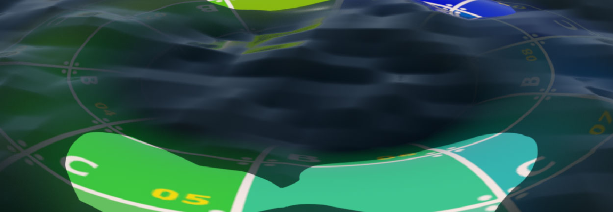
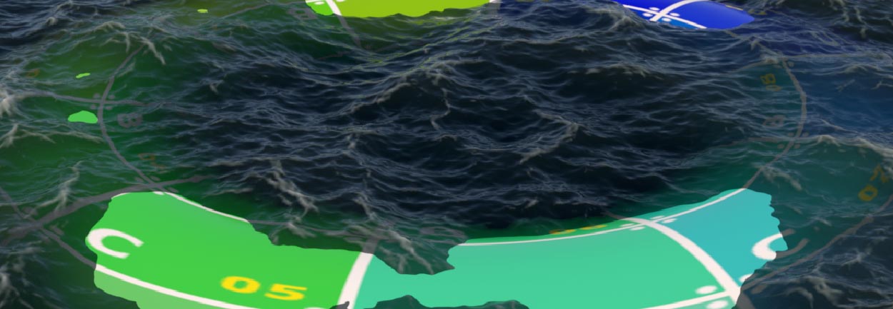
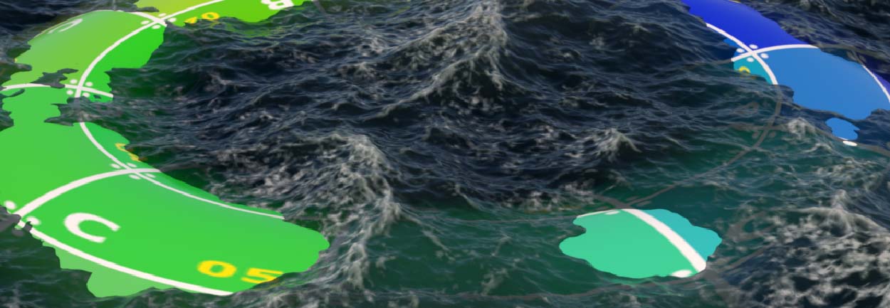
The network contains everything you need for an ocean, but still without a spectrum that generates the waves. When you go to the viewport’s render delegates dropdown and choose Karma CPU, for example, you will only see a flat and bluish-grey surface. Now, adjust the camera’s point of view to get a good view on your ocean. To do this, go the viewport’s second dropdown with No cam. From this menu, choose your camera - most probably it’s cameras/camera1.

This step is totally optional, but reference objects help us to get a sense of scale and relation. A nice byproduct is also that you can see the water shader’s absorption effect with a partially submerged object: the water becomes more opaque with increasing depth.

1. Add an object, for example a Torus LOP and place it between the physical sky and the render settings nodes to connect it.

2. Scale, rotate, and position the object to your liking, but make sure that it’s visible in the camera.

Here’s an example with a textured torus rendered with the viewport Karma CPU delegate. You can see parts of the torus as a narrow ring sticking out of the water. Also note how the object vanishes.

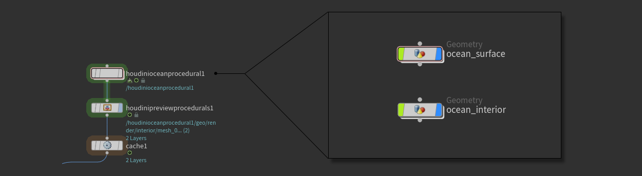
To turn the flat surface, shown above, into an ocean you need a spectrum. When you double-click the Houdini Procedural: Ocean node to dive inside, you can see two Geometry OBJ nodes: ocean_surface and ocean_interior. The surface contains networks for the actual ocean with waves and foam. This is the same setup you would use for a SOP-based ocean. The interior takes the render_grid Grid SOP and extrudes it to get a solid object.

1. For the spectrum, dive into ocean_surface and select the save_spectra ROP Geometry Output SOP.

2. Go to Output File and click the Open floating file chooser button. Then, define a file and a path for saving the spectrum. The file type is sc.bgeo.

3. Click Save to Disk to write the spectrum to the previously created file.

   You might have noticed that Valid Frame Range is set to Render Current Frame. The ocean procedural doesn’t require an entire sequence and a single frame is enough.

4. Return to the stage level and select the procedural node. On the Spectrum section you can see that Spectrum File already has a path to the previously saved file. That is because an expression fetches the path from the ocean_surface network. There are also expressions for reading out the spectrum’s evaluation time and the extruded geometry.

5. Go to the Dicing section and drag the camera1 node from the network to the Camera LOP Path field.

   If the viewport render delegate is already set to Karma, you can see a result similar to the image below.

   

6. To improve the ocean’s quality, go to the Geometry and increase Preview Quality, e.g. to 0.4.

Sometimes it happens that spectrum quality isn’t good enough or you just want to have a different wave pattern. You can reapply the spectrum and update the render geometry.

1. Dive into the ocean procedural’s ocean_surface context.

2. If you want to enhance spectrum quality, select oceansprectrum1 and increase Resolution Exponent.

3. If you want to create a different pattern, change Seed, for example. You can also open the Wind tab and create an entirely new wave surface.

4. Select the save_spectra node and click Save to Disk to overwrite any existing spectrum file.

5. Return to the stage and select the ocean procedural. Go to the Spectrum section and click Reload Geometry to update the Spectrum File.

With the improved quality, the surface should look similar to the image below. When you take a close look, you can guess whitecaps on some waves. The amount of whitecaps is controlled in the Shading section, where you can find various cusp parameters. Play with the values to create a more distinctive effect. Cusp Intensity, for example, controls the whitecaps' brightness. Values greater than 1 are allowed, but might create blown out areas. By default, Cusp Min/Max is turned on and creates a cusp PrimVar. You can use this attribute for shading and displacement of the ocean surface.

Aside from the cusp parameters there’s a Foam Particles checkbox. This parameter also expects a file path. In contrast to Spectrum File, where a single file is enough, Foam Particles requires an entire sequence: for an ocean sequence with 250 frames you also need 250 frames with foam particles. The foam particles are used to create a customizable foam pattern and appear as white spots on the surface.

The foam particles, however, are created and controlled inside Houdini Procedural: Ocean.

1. Dive inside the procedural LOP’s ocean_surface geometry node. There, select the oceanfoam1 Ocean Foam SOP node.

   The preadjusted parameter values are often sufficient, but it’s possible to change them, of course.

2. With Particle Density you adjust the amount of foam particles. More particles create denser foam marks on the surface. Note that particle counts can increase rapidly. For better control, consider opening the Solver tab and decrease Life Expectancy. Also note that it takes several frames for the foam to reach the maximum number of particles. It might happen that the first 15 or 20 frames don’t meet your expectations.

3. Another way to control particle counts is to use the parameters on the Conditions tab. Min Cusp measure the waves' choppiness. Only waves with a cusp level above the given values will emit foam. This is also valid for Min Velocity: ocean waves, moving faster than the parameter’s value, will create particles.

When you select the ocen procedural and take a look at Shading section, you can see three materials.

• Surface Material defines the look of the ocean.

• Interior Material is responsible for how light behaves when it travels through the water. Here you can control absorption and falloff effects.

• Proxy Material is used for the ocean’s viewport representation.

Click the Jump to operator buttons to directly go to the appropriate subnetowrks with the surface and volume shaders.

The Small Ocean shelf tool creates a surface of 100 m x 100 m and a depth of 10 m. To change this, you have to dive into the procedural again.

1. To change surface size, dive into ocean_surface and select the render_grid Grid SOP. There, use the Size parameters to adjust the ocean surface.

2. You can change depth inside the ocean_interior node. Select extrudevolume1 and enter a new value for Depth.

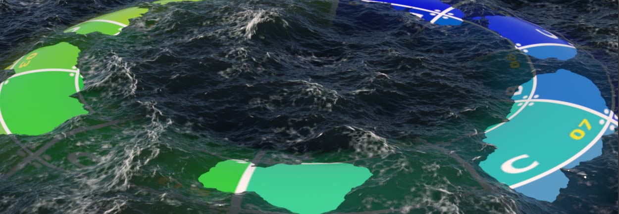
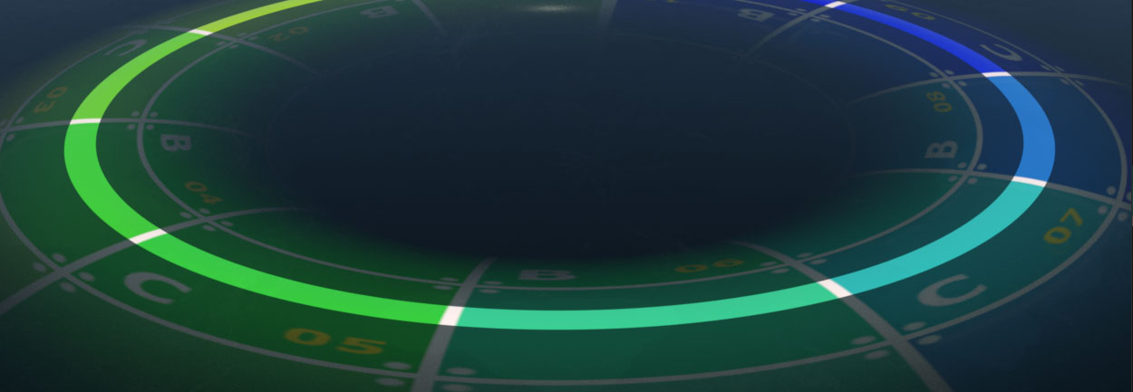
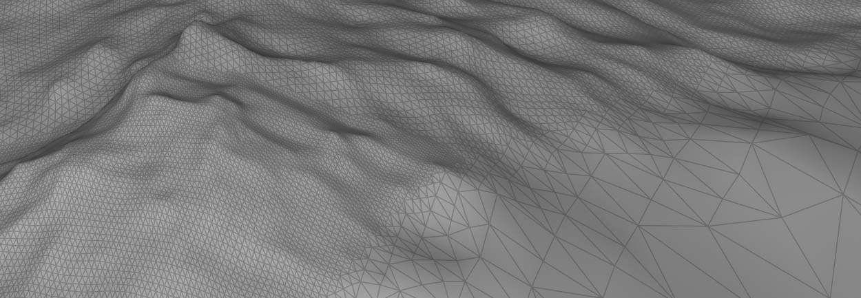
Highly detailed ocean surfaces can allocate a large amount of computer resources, but in many cases only a small fraction of the surface is really seen. Dicing is a method to dynamically change the level of detail based on the camera’s point of view: geometry outside the camera frustum has a low level of detail, while the ocean inside the frustum is displayed at full resolution. There is a smooth transition between the resolution levels. When you change the camera’s parameters, this transition zone will be recalculated. The image shows areas with different mesh resolutions along the camera frustum’s margin.

Without a camera, you will see a surface with just a few bumps. Only when both camera fields are filled in, all details will be displayed. Resolution should also match the resolution of the rendered image(s).

Downsampling is a very effective method to speed up the preview process, e.g. for evaluating the volume shader or the general look. The parameter decimates the spectrum data, but keeps all the other settings you've made. Depending on the Downsampling level you get a more or less coarse surface.

Rendering scenes with the Houdini Procedural: Ocean LOP doesn’t differ from Karma’s standard workflow. On the karmarendersettings node, make sure that you've

• chosen the correct Camera and Rendering Engine

• set a sufficient number of Path Traced Samples to reduce noise

• defined all AOVs on the Image Output ▸ AOVs (Render Vars) tab

• turned on motion blur settings on the Rendering ▸ Camera Effects tab.

Once you've made your settings, select usdrender_rop1 and choose a

• render method, e.g. Render to MPlay

• Valid Frame Range like Render Specific Frame Range.