| On this page |

The ![]() Houdini Procedural: RBD LOP is an alternative to the
Houdini Procedural: RBD LOP is an alternative to the ![]() RBD Destruction LOP that gives you full control over the import process. If you still want to use the destruction node as a higher level tool, you can do that. There you also have access to the procedural when you set Output Type to Procedural. However, the new procedural is the recommended replacement for the destruction LOP’s other Output Type modes like Deforming Mesh or Dynamic Skinning.
RBD Destruction LOP that gives you full control over the import process. If you still want to use the destruction node as a higher level tool, you can do that. There you also have access to the procedural when you set Output Type to Procedural. However, the new procedural is the recommended replacement for the destruction LOP’s other Output Type modes like Deforming Mesh or Dynamic Skinning.
In the past, users often had issues with bigger scenes. For example, large amounts of fractured pieces created an appropriate number of primitives. This normally lead to performance and naming problems, and the scene required (much) more disk space.
The Houdini Procedural: RBD is a separate tool that wraps up workflows from RBD/simulations and the USD side to solve the aforementioned issues. With this tool, the USD stage remains manageable and shows only the original primitives in the Scene Graph Tree.
When you simulate fractured geometry, the RBD solver also creates points that represent the pieces' transform information. You have one simulation point per rigid body. Instead of caching out fully animated geometry, you only save point data. The Houdini Procedural: RBD LOP will then connect the rest state of the pieces with the simulation points to restore the original transform at render time.
SOP setup 
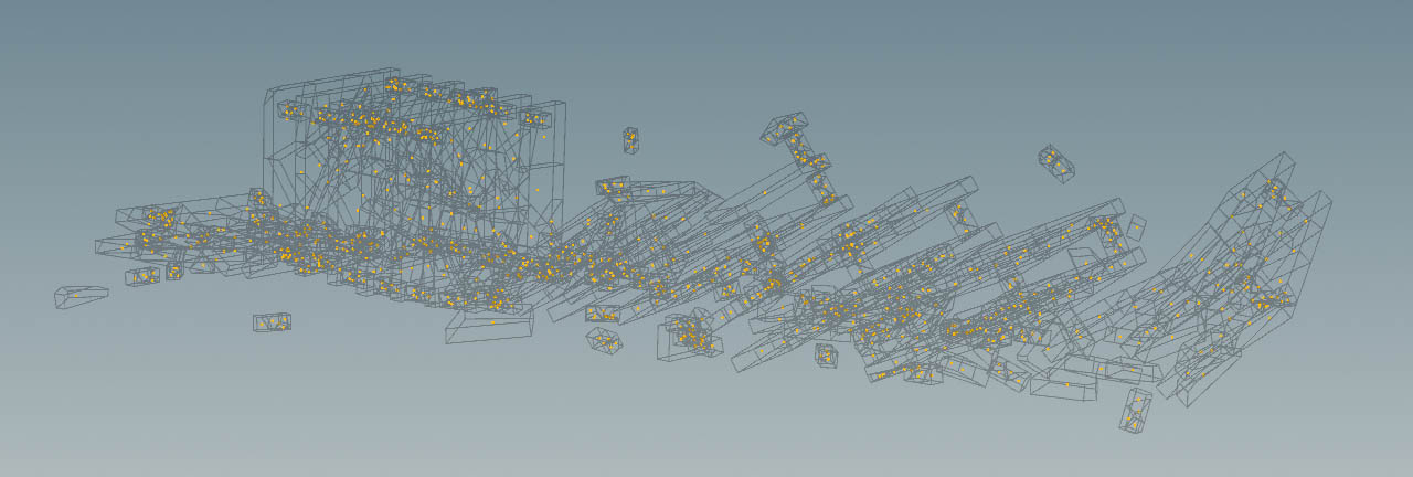
To illustrate the workflow, lets take a quick look at a basic RBD simulation setup. There, a prefractured tower falls down on a ground and breaks apart.
-
The SOP setup consists of an
 RBD Material Fracture SOP to break a hires object into pieces.The node generates points that determine, where the pieces are created. Alternatively, you can also connect already existing points to the node’s fourth input. Note that simulation points and fracture points are not the same!
 -
An optional
 RBD Configure SOP packs the input geometry and adds the relevant attributes to the simulation geometry (see the note below).
 -
The
 RBD Bullet Solver SOP performs the simulation.
Note
The RBD Configure SOP makes it easier to assemble a piecename point attribute. However, if you aren’t using proxy geometry, you would do this on the solver’s first input instead.

Attributes 
Attributes play a major role in conjunction with the RBD procedural, because they establish the connection between pieces and simulation points. To address the procedural, it’s necessary to perform a couple of conversions. Basically, everything is down to path and name attributes.
-
In Solaris, the
pathis the so-called USD primitive path and determines where in the Solaris scene hierarchy primitives will finally appear. The path attribute has precedence, but if it isn’t provided, thennameis used (and would typically contain a relative path which is appended through a Import Path Prefix on the SOP Import LOP).
To minimize the number of USD prims we also want to have a single
Meshprimitive for all of the fractured pieces. The solution is to assign the same path to the entire geometry. -
The
nameattribute is directly created by the RBD Material Fracture SOP and assigns a unique name to each piece, e.g.piece0,piece1, etc. This attribute is used by the Bullet solver to identify separate pieces, so we use thepathattribute to configure that all of the polygons should be imported into the same USDMeshprim.
The piecename attribute 
It’s not possible to pass name and path to the procedural directly, because they're already consumed by the aforementioned SOP Import LOP. This node loads the required geometry to Solaris. To overcome this restriction, you introduce a piecename attribute that is derived from path and name. The new attribute also avoids that you have to make changes on the default settings of the SOP Import LOP or your own definitions of path and name to control the scene hierarchy.
-
The
piecenameattribute must live on the pieces and the simulation points to specify which piece a certain point corresponds to. -
The
piecenamesimulation point attribute must be a full path and you can assemble it from the already existingpathandnameattributes. The reason is that the RBD procedural can handle multiple transformations simultaneously. The new path can be seen as a unique identifier.
Let’s say path is /world/tower and name is piece0. In this case, the piecename attribute’s resulting two flavors are:
-
Primitive →
piece0 -
Simulation point →
/world/tower/piece0.
Attributes: conversion 
The table below shows how the various attributes are modified when they pass the network nodes.
| Node | Action | |
|---|---|---|
|
|
Name |
Manually creates the path primitive attribute.
|
|
|
RBD Material Fracture |
Automatically creates the name primitive attribute.
|
|
|
Attribute Swap |
Renames the name primitive attribute to piecename.
|
|
|
Attribute Promote |
Converts the path primitive attribute to a point attribute.
|
|
|
Attribute Wrangle |
Assembles a piecename point attribute from path and name.
|
Attributes: path (primitive) 
Let’s start with the path primitive attribute. On the ![]() Name SOP, make the following changes:
Name SOP, make the following changes:
| Parameter | Value | Description |
|---|---|---|
| Attribute |
path
|
The name of the attribute you want to create. |
| Name |
/world/tower
|
The attribute’s value. Change this to your own requirements. |

Assuming that you work with the optional RBD Configure SOP, you have to make the path attribute accessible for the simulation process. On the Attributes ▸ Transfer Attributes parameter, change the default entry to v w path.
Attributes: piecename (primitive) 
The piecename primitive attribute is derived from the RBD Material Fracture SOP’s own name attribute. To rename the attribute, you can use an ![]() Attribute Swap SOP. Here are the node’s settings.
Attribute Swap SOP. Here are the node’s settings.
| Parameter | Value | Description |
|---|---|---|
| Method | Move | Renames the source attribute. |
| Class | Primitive |
In Solaris, a name attribute must live on primitives.
|
| Source |
name
|
The original attribute. |
| Destination |
piecename
|
The renamed attribute. |

Attributes: piecename (points) 
For the simulation points, you also need a piecename attribute. As mentioned in the introduction above, the points' piecename is a full path assembled from the name and path attributes.
Right now, path is a primitive attribute, but you need a point attribute. For the conversion you can use an ![]() Attribute Promote SOP and change the following parameters:
Attribute Promote SOP and change the following parameters:
| Parameter | Value | Description |
|---|---|---|
| Original Name |
path
|
The attribute you want to promote. |
| Original Class | Primitive |
The path attribute’s current type.
|

You also have tell to the RBD Bullet Solver SOP that it should transfer the path to its fourth output with the simulation points. Open the solver’s Output tab and go to Attribute Transfer. Change the default entry to age w path.
To assemble the piecename attribute you typically use an ![]() Attribute Wrangle SOP. On the VEXpression field, enter the following line of VEX code:
Attribute Wrangle SOP. On the VEXpression field, enter the following line of VEX code:
s@piecename = s@path+"/"+s@name;
Tip
The original name attribute is no longer required and you should remove it, because it’s rather heavy. You can do that with an ![]() Attribute Delete SOP at the bullet solver’s output. There, on the Point Attributes parameter, enter
Attribute Delete SOP at the bullet solver’s output. There, on the Point Attributes parameter, enter name.
Caching 
Caching is an optional step, where you write out the hi-res piece geometry and the simulation points to separate files. If you have heavy and slowly simulating scenes with complex fracturing, you should definitely think about fracturing. However, caching for the simulation points is necessary if you want to use the procedural’s File Cache ▸ Points Location mode.
You can use the ![]() File Cache SOP for this process.
File Cache SOP for this process.
Solaris setup 
Now that you have the required attributes, you can switch to Houdini’s stage level where you bring everything together. Let’s take a look at the network:

You start with a SOP Import LOP. This node was already mentioned in the Attributes chapter and it loads the pieces' rest state to Solaris. When you move the timeline slider, the objects should be motionless. The node also reads the path primitive attribute that comes with the pieces to establish the scene hierarchy. When you look at the Scene Graph Tree, you should see /world/tower. Additionally, the objects also carry the piecename primitive attribute.
Now, lets take a look at the procedural’s parameters. The descriptions in the table below explain the various settings.
| Parameter | Value | Description |
|---|---|---|
| Primitive Path |
/$OS
|
Here you define, where in the Scene Graph Tree the procedural appears. The default entry reads the node’s name (houdiniprocedural1) to create the hierarchy. You can change this path to your own liking.
|
| RBD Primitives |
/world/tower
|
This path must point to the pieces you've loaded through the SOP Import LOP. |
| Piece Attribute |
piecename
|
Here you add the name of the attribute that exists on the pieces and the simulation points. The default entry corresponds with the attributes you've created in the SOP network. |
| Points Location | Primitive |
The default entry reads the simulation points directly from the SOP network. This means that you have use the two associated Point parameters to a) specify where in the Scene Graph Tree the points appears and b) let the procedural know where to find the points.
With this option, it can make sense to add a With File Cache, however, you define the path to the file sequence with the points. |
| Point Primitive |
/rbd_points/$OS
|
Here you can determine the points' scene hierarchy. Again, the $OS variable takes the procedural’s name to complete the path. Change this entry to your requirements.
|
| Points SOP |
/obj/tower/POINTS
|
This is the SOP path to the particles. Typically, you create a |
When Preview Procedural is turned on, you can already evaluate the simulation in the viewport. You can also complete your stage by adding lights, camera, and everything else you need.
The Scene Graph Tree is now clearly arranged.
