Fast and Fracturous - Equinox
This presentation dives into what’s new in Houdini 21 for Rigid Body Dynamics, focusing on how the new nodes improve and simplify the existing workflows. We break down the different Car RBD workflows and show how these tools give you more control and flexibility when setting up vehicle destruction simulations.
You’ll also learn how to adapt these methods to different types of vehicles, helping you push the limits of what’s possible with RBD setups in Houdini. By the end, you’ll have a solid understanding of how to leverage these updates to create more efficient, realistic, and customizable simulations.
It is advisable to watch this presentation before diving into this tutorial in order to understand the process behind this project better.
The new RBD Car Fracture SOP and RBD Car Transform SOP, combined with the existing RBD Car Rig Tools in Houdini, make it quick and easy to set up a working car crash simulation.
This tutorial covers the full process:
- Rigging and driving two cars
- Fracturing them using the new tools
- Simulating collision destruction with the RBD Bullet Solver
We’ll walk through how the HIP file has been set up, helping you understand the workflow so you can either recreate it from scratch or build upon it. For the best experience, keep the HIP file open as you follow along. Click the "Download HIP File" button above to get the project files. With that ready, let’s get started!
STEP 1 - The Setup
It's important to start the rigging process with well-prepared geometry. This includes proper grouping for different parts, clear name attributes, and clean geometry—free of open faces, loose points, or interpenetrating meshes. While the RBD Car Fracture SOP can handle some topology issues, it's recommended to clean and prep the geometry for optimal results. Open the GEO_car_asset geometry node to view the car asset used in this project.
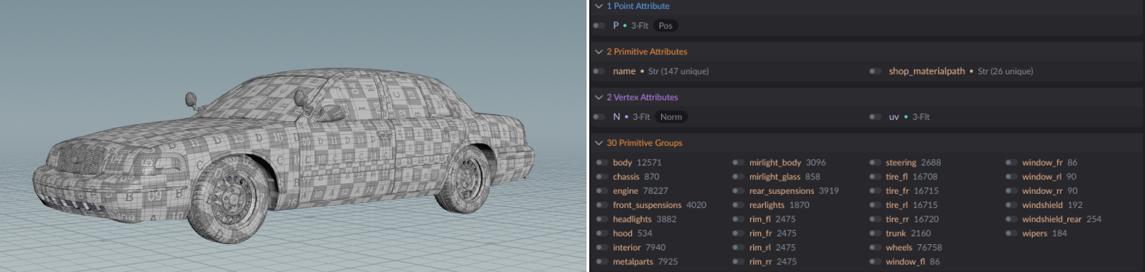
In this case, the car model already has proper groups, normals, UVs and a @name attribute. Generally, since the @name attribute will be overridden while fracturing the geometry, we would want to copy the original name attribute under a different attribute name or as a @path attribute to assign materials in Solaris. Fortunately, we have an existing @shop_materialpath attribute here that can be renamed to @path for the same purpose. Some additional steps include coloring parts of the wheels to better visualize their rotation and correcting the car body’s UV maps for later use while texturing in Copernicus. With that, we're ready to begin rigging.
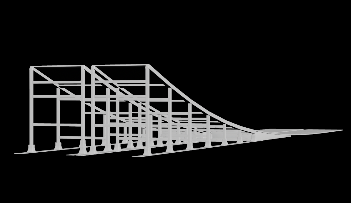
The project file includes several versions of the ramp geometry, as well as the ramp HDA. You can use any of the provided variants or modify the HDA to create your own—just make sure to install it beforehand. You can find the ramp in the GEO_procedural_ramp geometry node, along with the heightfield used as collision.
STEP 2 - Rig and Drive
Once the car and ramps are set up, we can begin rigging the car. In this example, the same car model is used twice, but the setup works just as easily for simulating multiple cars. Let’s dive into SIM_car_driving to see how it's set up.
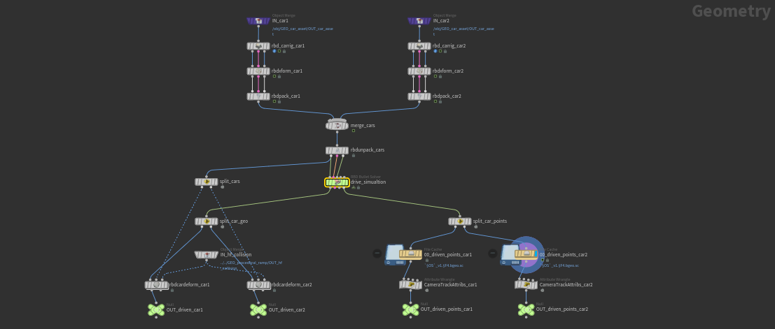
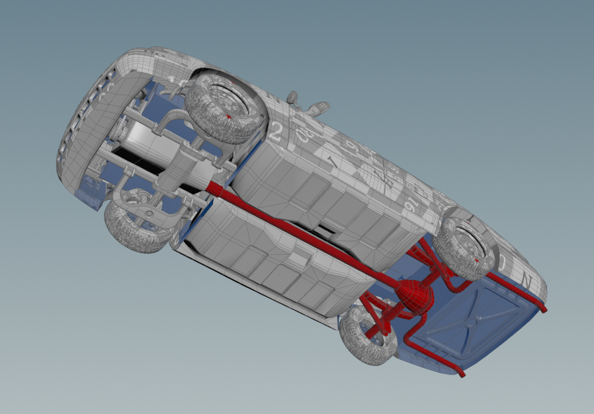
The RBD Car Rig SOP controls the driving parameters, while the RBDxform SOP sets the car's start position after rigging. We begin by assigning the Wheels Group and Steering Wheel Group in the car rig, and then animate the Steer, Speed, Brake, and Hand Brake parameters to shape the drive simulation. For more accurate results, we will configure additional settings such as Center of Mass, Acceleration Profile, Tire Friction, Wheel Scale, Suspension, and Density. Since both cars are identical except for the animated elements, all the parameters remain the same for each.
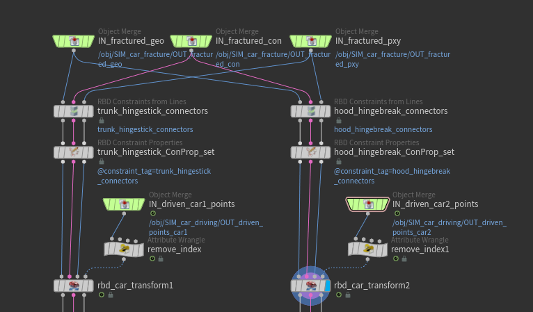
The cars are packed using RBD Pack SOP before merging, and then separated with RBD Unpack SOP by enabling
"Enforce Unique Name Attribute per Instance" and using the @index attribute. This ensures each car has a unique
name attribute, which is essential for the Bullet Solver to distinguish between them.
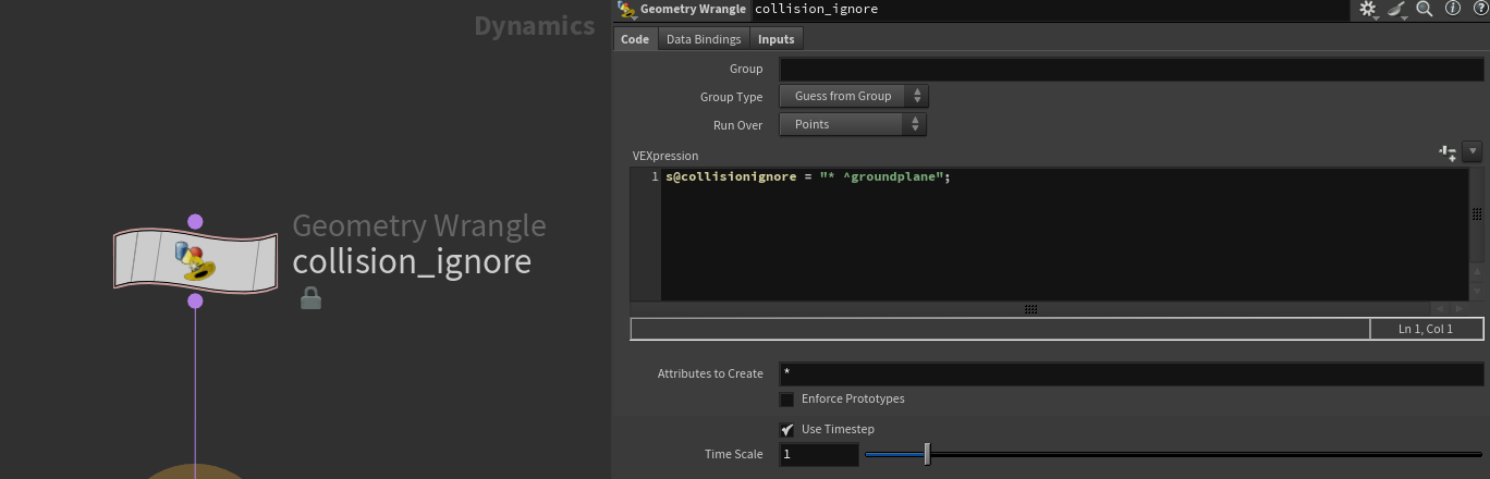
Geometry Wrangle used within the Bullet Solver to ignore collision between cars.
In the RBD Bullet Solver, using a Geometry Wrangle, collision is set to ignore everything except the ground plane to reduce simulation time by preventing the cars from colliding with each other. All we need as of now is for the cars to launch off the ramp and continue through the scene. The VEX code used is as follows:
s@collisionignore = "* ^groundplane";
Additionally, the @restxform attribute is output from the RBD Bullet Solver to transform the fractured geometry with the simulation points down the line.
In this setup, the ground plane is a heightfield that includes both the ramp and terrain. It’s prepared in the GEO_procedural_ramp geometry node and assigned as the collision object under the Collision tab in the RBD Bullet Solver.
The two main outputs from this process are:
- Simulation points—unique to each car.
- Deformed car geometry—with wheels and suspensions animated using RBD Car Deform SOP.
The same heightfield is used in the RBD Car Deform to ensure accurate deformations on the wheels and suspensions of the cars post the simulation.
STEP 3 - Fracturing
This is where most of the work will happen—but all within a single node. Inside the SIM_car_fracture, the same car used in the driving simulation, with the same RBD Car Rig (without any keyframes), is connected to a new RBD Car Fracture SOP. This preserves not only the names and constraints generated by the rig—crucial for the following simulation—but also key properties like Center of Mass, Tire Friction, Wheel Scale, Suspension, and Density, ensuring consistency throughout the setup.
We use separate Car Rigs to keep the driving and fracturing processes independent. This makes it easier to iterate on the driving—tweaking parameters like Speed or Steer—without needing to re-fracture the car each time. However, if significant changes are made to attributes such as Wheel Scale or Center of Mass, it's important to update this Car Rig and re-fracture the car to maintain accurate simulation results.
The first step is to set the Chassis Group. The chassis of this car is split into three parts: 'front_suspensions', 'chassis' (the exhaust in this case), and 'rear_suspensions'. For a frontal impact we want the front suspensions to break, so we will use only the 'chassis' and 'rear_suspensions', locking them as a single packed object that holds the wheels together. This setup allows us to fracture the front suspension separately.
If there are external objects like carriers or antennas that should be excluded from the simulation, we can specify them in the Ignore Group. Since we don’t have any, we shall proceed as is.
You must specify a Rest Frame and enable Re-Align Wheels if you have an animated car geometry. This will ensure that the heavy calculations aren't time dependent and that the wheels don't incur a double transform, respectively. Since we're fracturing a static car, we can leave the Rest Frame at 1 and the Re-Align Wheels disabled.
We will start by fracturing the front tires, as they will be squished upon collision. It is important to select only the tire geometry (the rubber part) for fracturing and keep the rims as is, so that the wheels remain attached to the car and the constraints coming from the Car Rig remain intact. By default, the tires will have 'soft' constraints without switching, enabling them to behave like 'rubber'.
We'll adjust the Fracture Density for more pieces and enable Edge Detail to break up the uniform voronoi pattern. One thing to note: when tweaking the Edge Detail parameters, the proxy geometry may start to behave oddly. To prevent this, avoid extreme adjustments or compensate by adjusting the Fracture Density accordingly.
Next, the process becomes straightforward in the Sections tab. We will assign different parts of the car to separate sections for independent control over the fracture type (metal, glass, wood, rubber). Aside from adding Edge Detail, enabling Proxy to Geometry provides an additional fracturing layer with varied fragment sizes. Constraint attributes like Strength Scale, Stiffness Scale, and Angular Stiffness Scale can also be adjusted per section but we're leaving them at default for now.
There is also a checkbox for enabling Constraint to Neighbor Sections. When enabled, it automatically links nearby sections using glue constraints.
It’s best to turn this off for parts like doors, hoods, or trunks that require manual constraint setups, such as hinge constraints. For metal, we'll use the Sheet model since these parts are planar geometry rather than solid objects. Despite being planar, the
RBD Car Fracture SOP extrudes the planes and converts them into solid objects when creating proxies. This extrusion can be controlled
by the Thickness parameter.
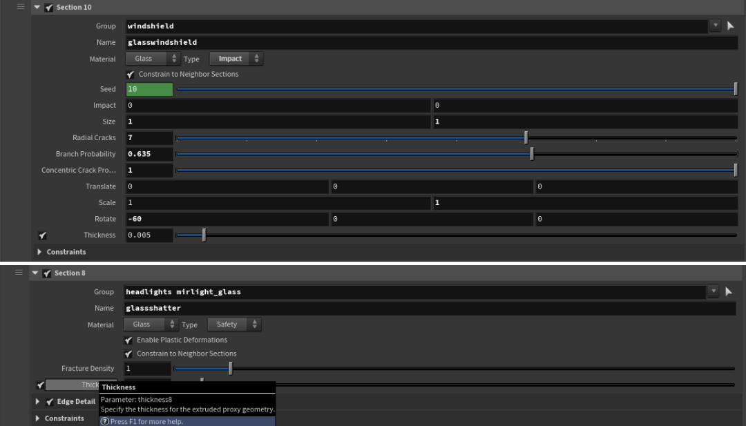
For the glass, we'll apply the Safety model to all windows except the windshield, for which we'll use the Impact model. This is a creative choice allowing the windshield to crack in a concentric pattern. The Safety model also has plastic deformations enabled, while the Impact model requires a more manual setup—since it only includes glue constraints by default. This would cause the glass to break immediately, but we want it to bend slightly first to reveal the concentric crack pattern. To achieve this, we override the constraints using an RBD Constraints Properties SOP to switch from glue to soft constraints down the line before simulating the crash.
If you check the Sections tab in the RBD Car Fracture SOP, you’ll see how the car is divided into different sections based on components and material types. For now, all section values are left at their defaults, except for Edge Detail and Constraint Color, allowing for quick iteration of the fractured car.
Additionally, you can control the Section Connector Constraints and global Constraint Attributes. The Strength Scale, Stiffness Scale, and Plastic Hardening Scale here affect all constraints between pieces and sections collectively. Since the suspension comes from the Car Rig, the Suspension Stiffness Scale can also be adjusted here, without needing to return to the rig each time. The values shown here were finalized after multiple test iterations, before caching the fractured car.
These constraint values can be adjusted at this stage or later using a separate RBD Constraints Properties SOP before the simulation. In this project we will do both. The Strength Scale, Stiffness Scale, and Plastic Hardening Scale is reduced significantly due to the high Constraint Iterations setting on the RBD Bullet Solver. With more iterations, constraints become harder to break unless their glue strengths are significantly reduced. This is where the global parameters become especially useful—they let us fine-tune all constraints across sections without having to adjust each one manually, streamlining the workflow compared to older methods.
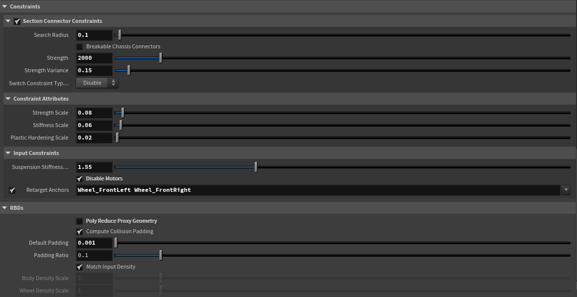
The Constraints tab and RBDs tab on the RBD Car Fracture SOP
We will enable Disable Motors to stop the cars from running after the crash, and turn on Retarget Anchors and assign the front wheel groups so that they break apart with the front suspension upon impact. This is necessary in this case because we’re dealing with a frontal collision, and parts of the front suspension are expected to break. Without retargeting, the wheels might remain attached to nothing, which looks unnatural. When retargeting is enabled, constraint anchors that were previously attached to the 'body' (the Chassis Group) are reassigned to the nearest fractured piece—since those pieces are no longer labeled 'body' . This allows the wheels to detach along with the broken front suspension and axle.
To optimize performance, Poly Reduce Proxy Geometry is enabled by default but we will disable it to avoid any volume loss errors that might occur, especially with smaller pieces. Compute Collision Padding can be adjusted here or in the Bullet Solver, and also helps prevent the same issue.
By default, Match Input Density is enabled to match the car’s weight as defined in the Car Rig. However, you can disable it and manually adjust the weight here if needed, without going back to the Car Rig. We shall leave it as is because the existing weight works just fine.
Here’s how the initial fracture looks after all these settings are applied.

Despite offering extensive control over sections and automatic constraint and proxy setup, this workflow can be further enhanced by diving inside the RBD Car Fracture SOP.
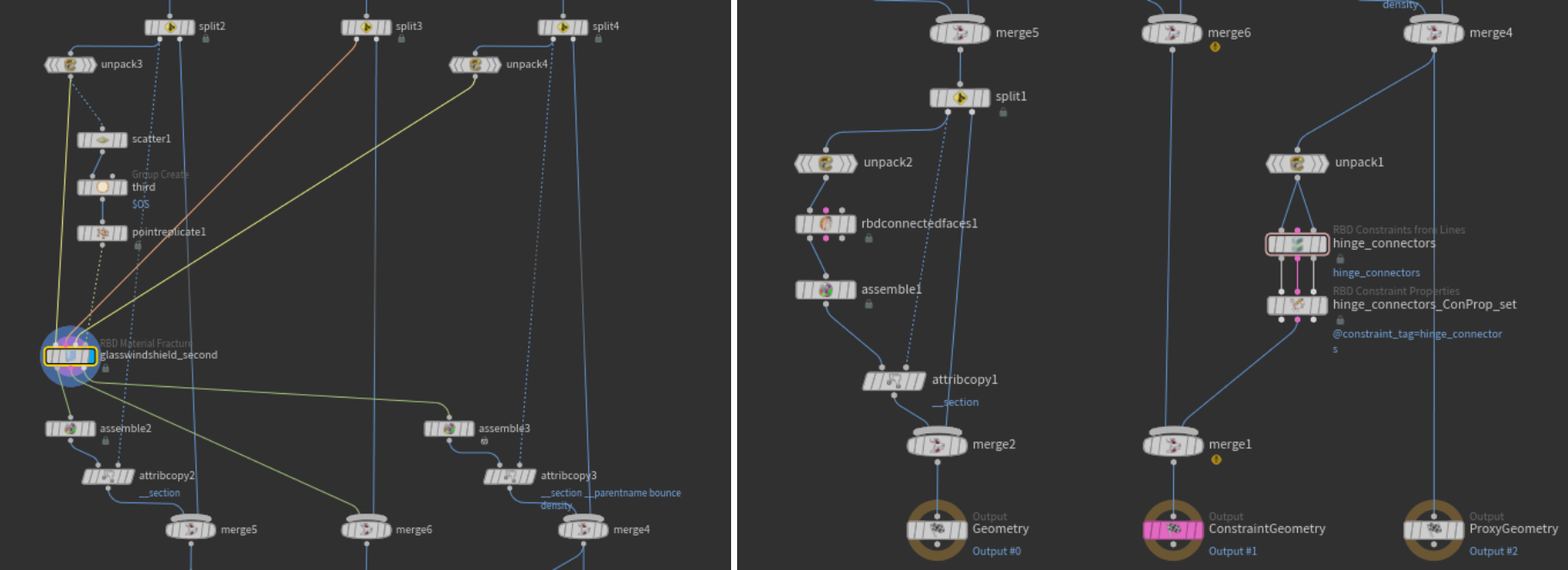
To add more detail to the windshield crack, we shall separate the windshield with a Split SOP and scatter points using the inside faces. Plugging these points into an RBD Material Fracture SOP for fracturing, helps preserve the existing setup. We will then copy the @__section attribute to the newly fractured pieces based on the @name attribute to maintain consistency.
The next important step is to set up the RBD Connected Faces SOP and enable the Opposite Face Name for both the existing inside group and the newly fractured pieces’ inside groups. Disable Create Constraints as it’s not needed here. This step is crucial for rendering fractured glass, ensuring that inside faces are revealed only upon breakage. After this, we will copy the necessary attributes again.
Parallelly, we'll set up hinge constraints for the hood and trunk. This allows them to pop open upon impact, creating a more natural movement upon collision. The hinge constraints should be set to Hard and Position Only to lock their position while allowing rotation around the hinges.
After the custom fractures and constraints are set, now is the time cache the car geometry using an RBD IO SOP. This way we can retain a single fractured version of the car while freely adjusting the drive simulation. Since the fracture setup is independent of the drive, we have the ability to iterate on the fracture after testing it in the crash simulation, as done in this case.
STEP 4 - Crash Simulation
As mentioned earlier, the Car Fracture SOP allows you to build further on the existing setup. At this stage, we have one fractured car and two unique sets of drive simulation points with the @restxform attribute and drive simulation data. Using the new RBD Car Transform SOP, we can drive the fractured car using these simulation points. Open the SIM_car_crash geometry node to follow along.
Note
Why use the RBD Car Transform SOP instead of Transform Pieces SOP?
The Transform Pieces SOP works by matching the name attribute on points to corresponding names on the geometry pieces. However, the drive simulation only provides 6 points—4 wheels, 1 body, and 1 steering—while the fractured car has many uniquely named pieces. The RBD Car Transform SOP solves this by using the @sourcename attribute on the proxy geometry, which matches the original name of the input geometry and that of the simulation points, allowing accurate transformation of the entire car.
Before plugging in the points, we will remove the @index attribute from the points, as it's not present on the fractured car. While you can recreate the @index on the fractured geometry and merge it later, it’s cleaner and more efficient to skip this step and instead use RBD Pack and RBD Unpack nodes downstream to manage and align the data.
Some additional constraints are setup in this phase to lock the hood of one car and the trunk of the other using more hinge constraints. This is to have them locked until a certain point in the simulation after which these constraints are deleted on the Bullet Solver to allow these doors to pop open.
Since this is specific to each car and is better to create on static fractured geometry, it is done right before transforming the car. Once this is done, we can connect the geometry, constraints and proxy along with the simulation points, to the RBD Car Transform SOP. This node has Re-Align Wheels enabled by default and it is necessary to leave this as is in order to prevent any sort of weird rotations on wheels during the crash simulation.
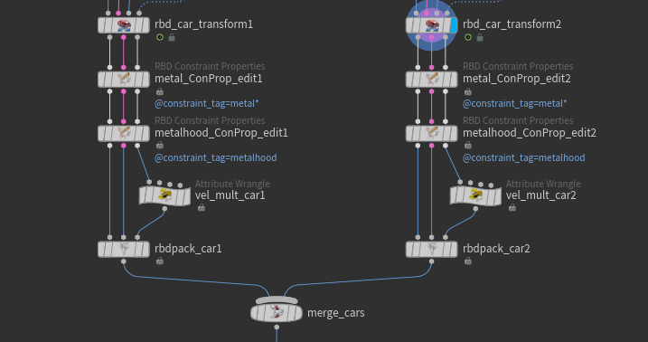
We shall perform other car-specific operations, such as editing constraint properties on individual sections before packing and merging. In this case the overall metal constraint strength has been tweaked independently to make one car more rigid than the other. Additionally velocity is manipulated using a simple VEX expression: v@v *= chf("Multiplier");
This creates a float parameter that multiplies the velocity by the specified value. It's used here to make one car push into the other and penetrate upon collision.
After that, both cars are packed and merged—just like in the drive simulation phase.
Adjusting the constraints created in the RBD Car Fracture SOP based on requirement
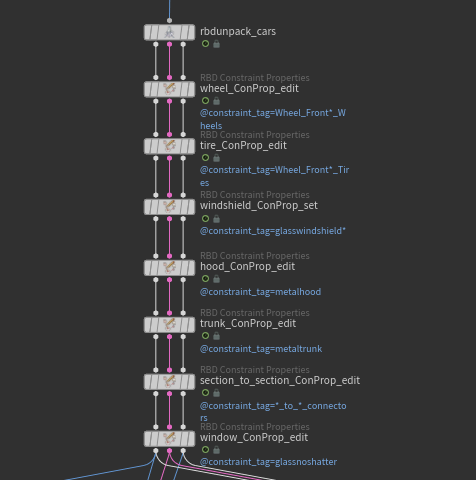
After unpacking, we'll modify constraint properties common to both cars. In this case, the following adjustments have been made:
- Glue strength has been increased on the wheel constraints.
- Angular damping has been adjusted on the soft constraints of the tires.
- Constraints of the windshield have been redefined.
- Angular properties of the hood and trunk door constraints have been tweaked.
- Strength of the Section Connector Constraints and window constraints has been increased.
(All these adjustments are specific to this setup and were refined through multiple iterations of the crash simulation.)
Right before simulation, the cars are split and frozen at frame 1 using a Timeshift SOP. These will later be used in the RBD Car Deform as reference inputs for deformation.
Separately, both cars are also frozen at the simulation's start frame to be cached as high-res geometry, which will be transformed using the Transform Pieces SOP with the simulation points. Why? Because we have points with unique name attributes corresponding to the name of each piece. This approach reduces the need to cache heavy geometry to disk.
Since constraints cannot be transformed like geometry--because we are setting them up for deletion on the Bullet Solver--they must be cached separately alongside the simulation points. Retiming the simulation for slow motion is a requirement, so it is we will cache more substeps to disk for better accuracy.
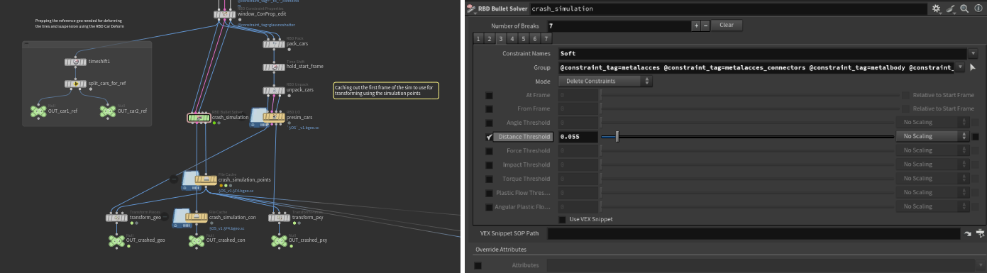
Most of the key work happens under the Constraints tab on the RBD Bullet Solver. Here, we'll select constraint groups using the @constraint_tag attribute and delete the constraints either based on a threshold or at a specific frame. This gives us fine control over how the cars break apart, allowing for more art-directed destruction.
For example, in the image above on the right, all metal constraints—which are soft constraints—are selected and set to be deleted beyond a threshold of 0.055, causing impacted pieces to break off and fly apart, adding a more dynamic feel to the simulation. You can explore all the tabs under Break Thresholds to see how these are configured—it’s all fairly straightforward.
Beyond that, several other parameters help improve the simulation:
- Constraint Iterations have been significantly increased.
- Collision Padding is set for both piece-to-piece and geometry-to-collision interactions.
- Drag is enabled to help stabilize the motion.
- Randomize Constraint Order is turned on to improve stability.
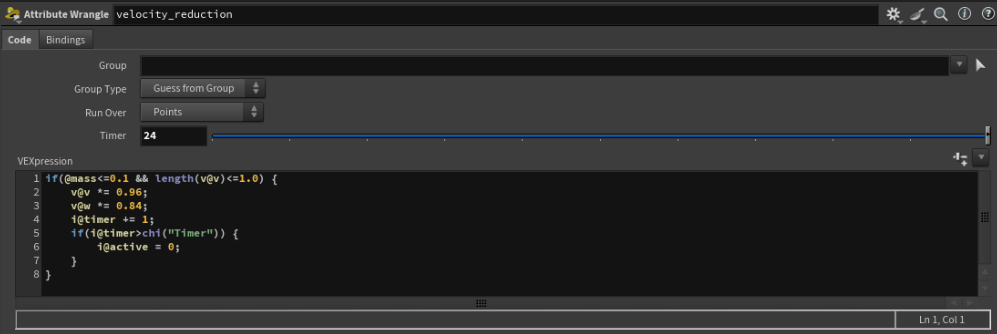
A common issue with simulating very small pieces is that they don’t settle easily and continue to jitter. This happens because their mass is extremely low—well below 0.1. To address this, we read the computed @mass and @v of each piece on every frame using a SOP Solver within the RBD Bullet Solver. Using an Attribute Wrangle, we multiply the @v (velocity) by 0.96 and @w (angular velocity) by 0.84 to gradually reduce the movement if a piece has @mass less than 0.1 and @v less than 1. Additionally, we start a @timer for these pieces, and if the timer exceeds a value of 24, we deactivate the piece entirely so it no longer moves.
When it comes to caching the simulation, we will only cache the simulation points and the constraints with 10 substeps each. Since we have already saved the static fractured cars to disk, we can use these simulation points with the Transform Pieces SOP to transform the fractured cars. But why do we need to cache substeps? This will be explained shortly before which we will take a look at the FARM_cache TOP on the object level.
This TOP setup was used to run all simulation caches using the render farm. This is an efficient way of running multiple simulations while still continuing to work on the current file. If there isn't a farm to leverage, this PDG setup can still be run using the Local Schedular. Additionally, you have the option of setting up wedges for any of the parameters you want to iterate on. Although this hasn't been done here, it is an option you could try at your own convenience.
A requirement for this project is to retime the crash simulation to create a slow-motion effect. This is where caching substeps becomes important. When you retime simulations directly from the solver, the sub-frame data (the information between integer frames) is still available. This allows the Retime SOP to interpolate smoothly between frames, producing accurate slow-motion results. However, once a simulation is cached to disk, the default behavior is to store only a single substep per frame. This means the sub-frame data is lost, preventing proper interpolation. To fix this, we need to cache multiple substeps. Caching substeps for geometry can be quite heavy on disk space, so instead, we cache substeps on the simulation points output from the Bullet Solver, which is far more efficient while still preserving all the necessary information for retiming.
Since we set the constraints to be deleted beyond a certain threshold, it is not possible to transform the constraints using these simulation points like we can on the geometry and proxy. This is why we have to cache the constraints with the same number of substeps as the points.
Now let's open the POST_retime_for_slomo geometry node to see how the RBD simulation is retimed.
STEP 5 - Retime and Deformations
The deformation process has been significantly simplified. The RBD Deform Pieces SOP and the RBD Car Deform SOP are the two main nodes to focus on. However, before deforming, we need a slow-motion version of the cars for the final output, so it’s wise to use the Retime SOP before deforming the geometry.
Using the Retime SOP, we’ll stretch 5 frames from the start of the simulation, to 50 frames. Retiming by frame range is a good option, as it gives us an exact 90% speed reduction. This same factor can later be applied to the time scale of all secondary simulations like debris and dust.
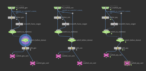
Since the cars won't move after the specified frame range, we switch to a Timeshift SOP that has offset the normal speed sim to start where the slow-mo ends. Now that everything from the frame of impact to the end is covered, we still need the data before the frame of impact. This is where the next Switch SOP comes into play switching from the actual cache to the slow-mo. This is repeated on the constraints and proxies after which the two cars are split based on the @index attribute.
After splitting the two cars into separate streams, we can perform individual deformation operations. This allows for manual adjustments to each car, such as post-impact animations. Let's dive into the POST_car_deformation geometry node to take a look.
The RBD Deform Pieces SOP requires three inputs: geometry, constraints, and proxy geometry. The Group must be set using the @name attributes created during the fracturing stage. Since we only need to deform metals and rubbers, it's best to have named the parts accordingly (e.g., metalxyz, rubberabc, etc.) on the Car Fracture SOP itself. Set the Group Type to Points, and the Boundary Connection to Cluster Attribute and Constraints. This ensures that pieces with deleted constraints don’t remain deformed but instead break apart correctly. Set the Cluster Attribute to @parentpiece. Finally, for the RBD Car Deform SOP, use the reference geometry output from before the crash simulation as the second input.
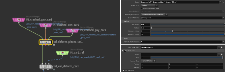
Make sure to set the Chassis Base Group on the RBD Car Deform SOP to @name=body-(@index) based on the index of your car, in this case 0 or 1.
After unpacking the output geometry, we need to use the RBD Disconnected Faces SOP to re-enable the @oppositefacename attribute and also create a @disconnected attribute. This allows us to delete the inside faces based on that attribute and also use it to scatter points on the inside faces for sourcing glass debris.
One of the problems with using an asset that contains interpenetrating geometry is that, although the Car Fracture SOP can
still fracture it, the simulation may produce unexpected behavior in
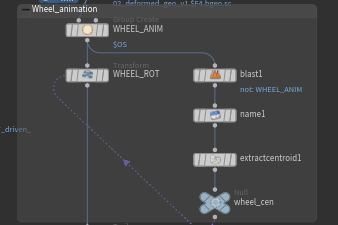
certain pieces. In this case, the front left wheel—which is expected to
spin since it doesn’t receive much impact—fails to behave correctly
because it collides with other geometry that intersects the tire. A
simple fix for this is to isolate that wheel and manually animate it
based on the overall movement of the vehicle.
After addressing this, the next step is to clean up any unnecessary attributes and groups, and compute velocity on the deformed geometry. Since we use the fractured version of the cars only from the frame of impact onward, we can blend it with the non-fractured car from the drive simulation up until that point.
All that’s left is to use the simulation geometry to source and simulate secondary effects like glass debris, glass dust, car dust, ground impact dust, and tire trail dust. This HIP file contains some intermediate-level setups for these secondary simulations. These setups are reusable and can be simplified or expanded into more complex versions based on your needs.
While this tutorial focuses on the destruction effects, the file also includes a Solaris setup. This covers assigning materials to the cars and secondary sims, adjusting textures using Copernicus, setting up wedges for different scene cameras, rendering layers, and compositing them in Copernicus. Feel free to explore the file—break it down, study it, or rebuild it from scratch.
Related Links
CREATED BY

COMMENTS
Qwame 3 months ago |
Thanks for this tutorial. Please when are getting a video tutorial on this subject?
moshvisuals 2 months, 1 week ago |
It is not a tutotial but is a step by step of what is in this post.
https://www.youtube.com/watch?v=aiRL_0sz1zw
moshvisuals 2 months, 1 week ago |
This great, just what I needed to fully understand this two nodes.
Viswesh Rameshkumar 2 months, 1 week ago |
Glad it helps!
Please log in to leave a comment.