CUSTOM ORIENTATION | CHAPTER 2 - CLIP 2

Transcript

Hello and welcome to the second clip of chapter two. In this clip, we continue with the curve that is not yet finished with its orientation, and we still don't have applied a role. The roll is supposed to give us that nice cinematic look that kids like these days.

So we bring in what we did in the last clip with another merge, without making a mess with additional wires.

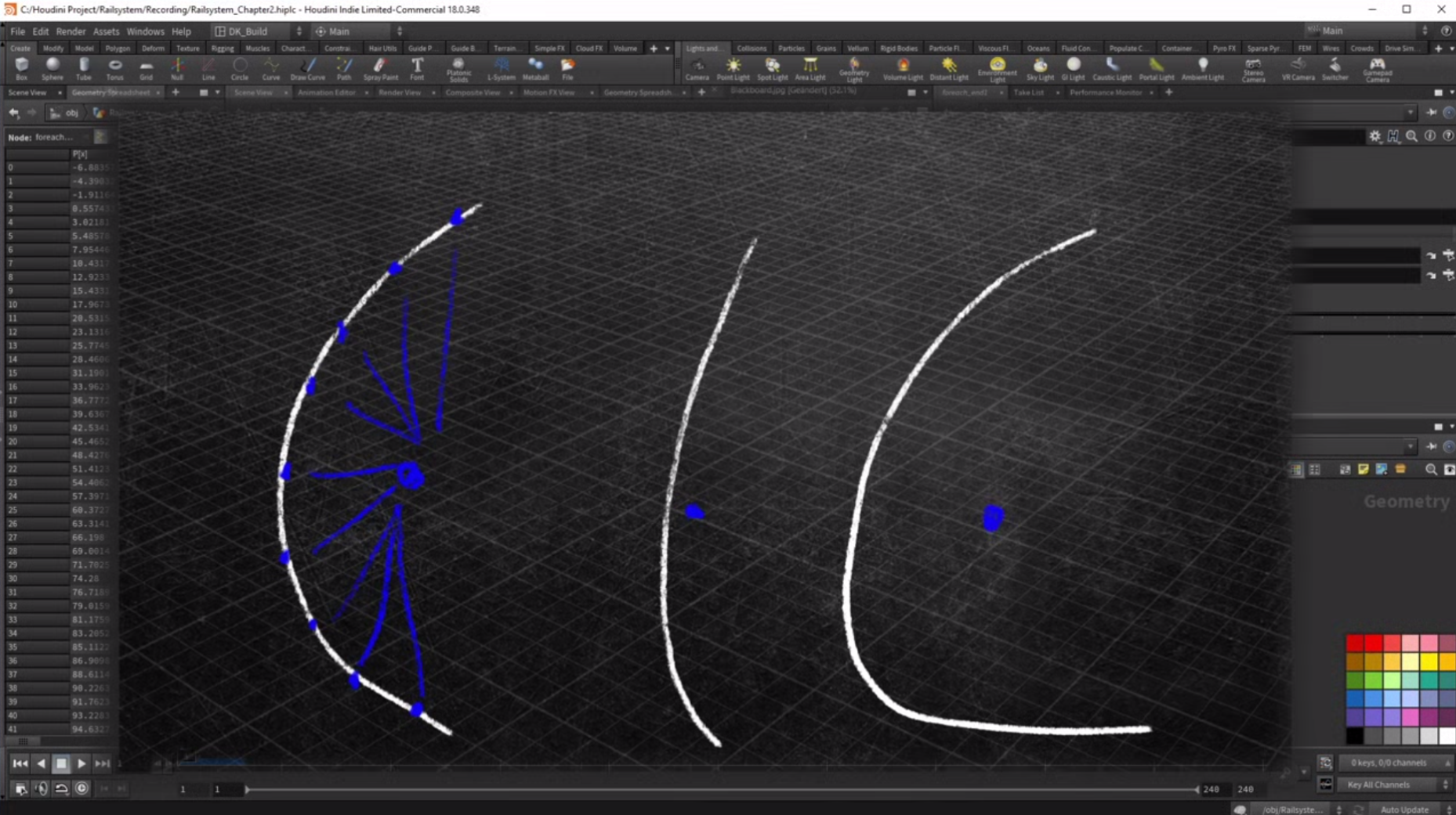
Then I am using a blast to isolate only the points that are in a lean group at the moment. That's all of them. That also creates a problem. Since I want to look at each piece of one group at a time. This roll should only happen in these groups. So we have to make sure that only those two groups go through this section to look only a connected segments.

I need to know what is connected for that. We can use the connectivity node, which we directly feed into a for loop. We are going to make sure that the individual left and right groups are not connected later. The connectivity creates an attribute that is placed on whatever it runs on. Let's turn it to primitive and call it segment.

And that's the same name you need to use in the end block of the loop. I did that by hand to show how they are connected, but you could have also used the, for each connected piece preset, which would have created the connectivity node for you. Now with that in place, let's look at a specific piece to demonstrate what should happen.

Let's see where the different areas are. We might want to look at this part in the lean right group. This will have a strong lean factor, which is a shame since it will happen in a tunnel, but it is a good example.

Figuring out a factor to determine the amount of roll I want on each piece could be achieved in multiple ways.

Now, if we add all the positions on this line together into one vector and divided by the amount of points used, we actually get an average of them all. And that point would have a very obvious factor on it. If it is a small turn, it will be close to the original curve. If it is a strong term, it will be farther away. And that's what we are going to do.

Well, okay then that was not so hard after all.

Then now let's write that in facts.

Good God

To do this, We are going to need to different vectors. One that will hold the result. And another one for the individual positions, we need to add them together.
So we are going to loop over them.

This, by the way is a typical scenario where you should use a wrangle set to detail. A point wrangle in itself is already a loop, but you don't have access to other iterations on a detail wrangle. You create the loop yourself, which then allows you to do something with the result. Inside of the loop. We grabbed the point using the counter variable.

When you think back to the sketch, it looked like the line was on the same level, but in the terrain, the curve could be all over the place.That's why I set the Y component to zero. Then just add the vector to the overall vector.

Once the loop is complete, we divide that overall vector by the amount of existing points. I definitely want to see this point in the viewport. Just to make sure that it is working. And there it is, sitting on the zero plane as it should. But as you can see, the curve itself is not to get an accurate measurement. I am creating a separate stream where I first set the position to zero. That way I don't interfere with the original position. I connect the modified curve into the second input.

Back in the wrangle - I can now get the distance between my average position and the closest position of that curve. Once I have the point and the distance I am going to give that point, a sign. I give it an attribute called marker set to one.That way I can easily find it in the next step. The distance is also going to be saved. As an attribute.

And again, you might be unsure if everything worked or you are still experimenting with ideas, don't hesitate to throw around with attributes.

Yes. Having a lot of unnecessary attributes can slow down your project, but you can always delete them when you are done with them.

I did use the attribute again for the lane factor, but we can get by without it. We see that in a few today, you can simply throw down a node called Oriental long curve and you are done with that. You can even let the node create the orient attribute, but the orientation was just the first task. I want the train to have a custom twist that I can control. So let's head back to our test marker. Each part of the curve is going to get its own custom factor.

Since we are dealing with curves, I decided to misuse the curveu attribute, usually that's a point attribute holding the value zero to one, displaying the points position on the curve. That will be my starting point as well. So we divide the current point number by the amount of points using Cast to float. So we have values with decimals, take a look at the spreadsheet and you will find the new attribute here.

Next, I use a technique I like to use to remap the range first, multiply by two. Subtract one, and then multiply the attribute by itself. Now we have a range starting at one, going down to zero at the center and end up at one. Again, you get a better idea on how this works. If I comment these lines out and add them back in one by one, this is extremely useful. When you want to do custom bend operations, we will see that later doing the course as an additional note, we multiply the value by itself to get rid of the negative values.

You could do the same with the absolute function. I want a twist that slowly builds at the beginning and reaches the maximum in the middle.So I need to reverse the values.Now, the curve you attribute begins at zero and ends with zero. Well, not quite the last point seems to not reach zero. And that's because I forgot to reduce the point amount by one. Again, taking into account that the point started zero.Now it fits into the range.

Are you really trying to downplay that? You already forgot what you tried to teach yourself? Only a few recordings ago.

If we wanted to be nitpicky, we would have to reduce the amount by two. The last point is still the marker point. To be honest, it is not the best way to have the special point, the marker in the same geometry as the curve, we could have separated them, but this gives me the opportunity to show you a good application for the find attribute malfunction.

That's more like it for gov, but pretend it was all planned that way. With this function, you can find points that have a specific value in an attribute here. I want to find the marker. I am looking for a point attribute with the name marker and the value I am searching with is one.

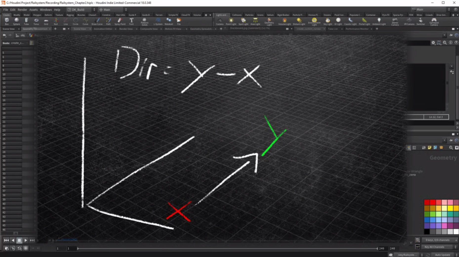
We only have one marker.So that is the returning point number, very handy. Now that I got the point number, I can also read the distance attribute I created finally for my test. I need a vector pointing from the curve towards the marker. If the vector has a pure direction purpose, it is always a good idea to normalize it. And you remember the cast of vector?I am sure this is another example of vector math. That you will need again. And again, if you have two points in 3D space, let's call them X and Y often you need to create a vector that points from one point to the other.

We know that the two vectors are pointing into opposite directions. Now we decided to use the orient a long curve node. That means the attribute my by tangent does not exist, but all it really was, was a cross product between the tangent and the up vector. In this section, we have a negative value. Let's take a look at a section with the opposite turn here. The turn is a lot smaller.

You can see how the marker direction just barely breaks of the main curve. But now that we confirm that it does work, we can get rid of all the extra attributes. Just turn them into simple variables.We already have the curve you attribute. But we need to negate the value.

If the dot product is negative as well.
And finally, I want to have a multiplier to control the attribute for that. I remap that distance to the marker from whatever it is to go from zero to one. Then I just multiply the curve. You attribute with that.

So let's test what we have done so far. We need to increase the max channel of that multiplier to see the effect.When we go into the double digits, we start to see changing values on the curve. You attribute let's switch to the stronger term. This is a good example to fine tune the settings, to get what we want. But even though it is helpful to see if the numbers in the spreadsheet change, as we expect them to do.We should look at something else to find the right values, but first let's get rid of the marker point. It has served its purpose.

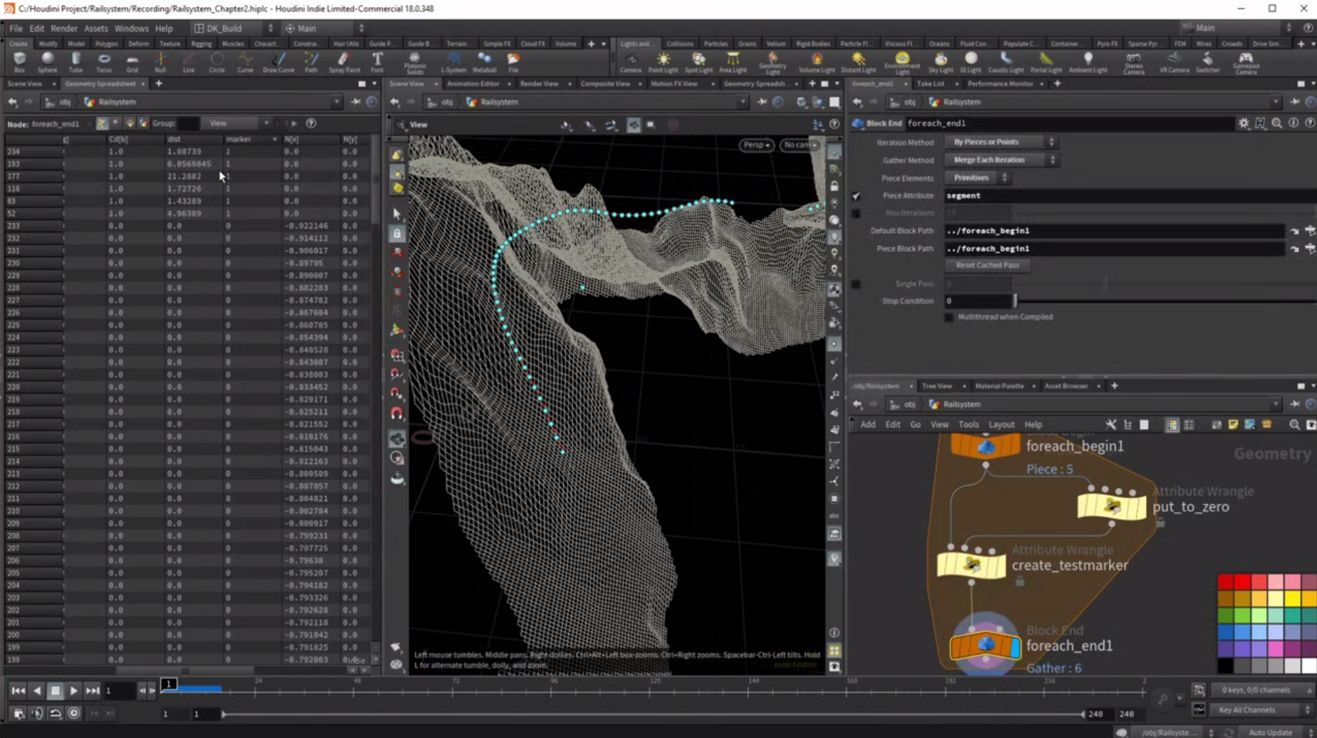
Just throw down a blast node and select whatever point has the marker attribute set to one.As I said, all points are currently in either the left or the right group. That means the whole curve is still connected. We need to add something to the system to actually cut that connection rather than directly jump to left or right. I want to add a threshold that needs to be exceeded for a group affiliation.Now you can identify the sections that don't have a meaningful turn by having even the shortest part of the curve in between both groups, they are not connected anymore. Now the connectivity node creates more segments and we loop over each of them creating a test marker for each piece by itself, we established a custom attribute.But now we have to actually apply it to the curve.

First. We just need to get the attribute on it. Throw down an attribute transfer note. We want to transfer the created curve. You attribute from points to points. This node works with proximity. Since the points are the same, we should get an accurate copy.

At this point, I want to rename the curve. You attribute something more obvious.The curve you attribute now becomes the role attribute.I am about to use another orient, a long curve node, but this time I am using an additional option on that node.

First let's connect the boxes again. We have orientation, but no leaning yet.Now create the orient node again, activate the orient, attribute the difference this time is that we want to apply, roll and twist. When we change the partial twists slider, you can see how it will affect the rail, but I don't want to set it to a fixed value. I want it to be defined by that attribute we created.So switch the option to scale by attribute. The default name is already role. With the copied boxes, we can now actually see how our custom attribute will behave while a value in the sixties will result in a strong roll. The same value does not really affect the smaller turns. You would have to really push the value to get a feedback in these areas, but that was the intent.

The roll effect is now dependent on strength of the turn.Let's close this clip with some cleanup, we created a bunch of groups and attributes that we don't need throw down a clean sob, and we get rid of the lean groups and we don't need the color data and the curve you attribute anymore. That's also a good place to throw down another output.

No, now we have a truly oriented curve.After we did some work on the node tree layout, we can take a closer look on the current status of the control node. At this point, I transferred all important parameters to it. Most of these settings concentrate on the height level of the rail. With these settings, you are able to find the perfect fit between the base level and the surface.

The other parameters define the role behavior. How much or less role we get on a given term. Now with the curve prepared, we can look into actually shaping the rail for this. I am going to apply the super formula, but that's for the next clip.

You heard it. The next clip is coming and it uses the almighty super formula, whatever that might be.
Let's find out in the next clip and

Hit the subscribe button for God's sake.