| On this page | |
| Since | 18.0 |
Overview 
The Pyro Solver is a wrapper around a DOP network to simplify the running of Pyro solves.
Note
The interface has been redesigned in Houdini 19.0.
Inputs 
Volumes for Sourcing
Provides the sources for the Pyro simulation. This should be a set of named volumes. The exact names required are determined by the Sourcing tab. The ![]() Pyro Source SOP and
Pyro Source SOP and ![]() Volume Rasterize Attributes SOP are useful tools for creating source volumes.
Volume Rasterize Attributes SOP are useful tools for creating source volumes.
Volumes or Geometry for Collision
The second input provides the collisions for the Pyro simulation. It should be a SDF VDB, such as the second output of the ![]() Collision Source SOP or the main output of the
Collision Source SOP or the main output of the ![]() VDB From Polygons SOP. If the collision is animating, points with a
VDB From Polygons SOP. If the collision is animating, points with a v attribute can be used to describe the motion. The two outputs of the ![]() Collision Source SOP can be merged and used as the second input to provide this.
Collision Source SOP can be merged and used as the second input to provide this.
Parameters 
Reset Simulation
Clears the entire simulation cache. Ctrl-click to also jump to the start frame.
Start Frame
What frame on the Houdini playbar that the simulation should begin at.
Quick Setups
This menu lets you run some simple scripted setups to help with the most common tasks.
Initialize Sources
Populates the Sourcing tab based on the incoming volumes.
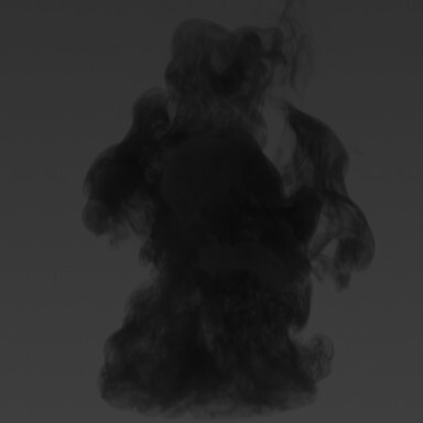
Initialize Smoke
Initializes the solver to simulate smoke.
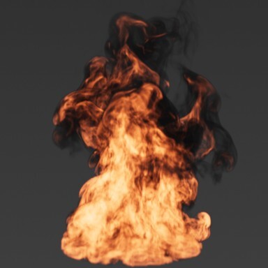
Initialize Fire
Initializes the solver to simulate fire.
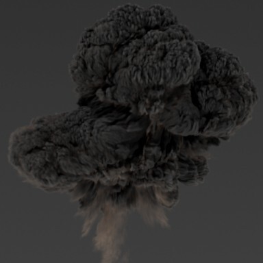
Initialize Explosion
Initializes the solver to simulate an explosion.
Add Color Source
Creates an additional source for working with color volumes.
Reference Bound
Creates a ![]() Box with the same dimensions as current size of the pyro domain. The Size and Center will then reference the parameters from the box.
Box with the same dimensions as current size of the pyro domain. The Size and Center will then reference the parameters from the box.
Setup SDF Collision
Sets the Collision Type to SDF + Volume Velocity and creates the necessary nodes to convert the geometries on the second input to volumes.
Create Pyro Look
Creates a ![]() Pyro Bake Volume that lets you further refine the look of your pyro simulation.
Pyro Bake Volume that lets you further refine the look of your pyro simulation.
Create Lights
Creates an Environment and a Directional Light at the object-level with a selected preset. This is useful to quickly create lights to improve the look of the pyro simulation in the viewport.
Create Lights/Cameras
Creates all necessary nodes to quickly get you started with rendering in Mantra. This includes environment and volume lights, as well as a mantra render node. It also enables motion blur on the render target (Geometry Velocity Blur in the Render → Sampling tab of the object-level node).
Create Render Stage
Creates all necessary nodes to quickly get you started with rendering. This includes environment and volume lights in LOPs with Karma. When looking through a camera upon selecting this entry, the selected camera will be imported to LOPs. Otherwise, a new camera will be created based on the viewer’s position.
Cache Simulation
Creates a ![]() File Cache node that is setup to cache a pyro simulation.
File Cache node that is setup to cache a pyro simulation.
Setup 
Voxel Size
The size of a voxel in the Pyro simulation. Cutting your voxel size in half will require eight times the memory and time, so a careful trade off between detail and pragmatism is required.
Velocity Voxel Scale
This multiplier is applied on top of Voxel Size to determine size of velocity voxels. Larger values of this parameter thus correspond to lower- resolution velocity fields, which will simulate faster but produce less detail from the motion.
Note
If Velocity Voxel Scale is slightly larger than 1, then the
simulation is unlikely to run faster; in fact, it may slow down due to
requiring slower sampling. To measure a performance benefit, the slower
sampling must be sufficiently offset by data reduction in the velocity
field. To this end, Velocity Voxel Scale should be set closer to (or
larger than) 2.
Time Scale
A scaling factor for time inside this solver. 1 is normal speed, greater than 1 speeds up the simulation, while less than 1 slows it down.
Simulation Type
By default, this solver operates in sparse mode; that is, the needed calculations are performed only in the areas of interest, as governed by the active field. Dense on the other hand performs a full global solve everywhere within the domain. Change this to Minimal OpenCL to enable a fast, dense solve using your graphics card.
Sparse
Calculations are performed only in the areas of interest, as governed by the active field. This region is built by looking at the Reference Fields parameter under the Bounds tab: positive areas of the specified fields are flagged as active. This intermediate active region is then dilated to provide a buffer for smoke to expand into. With the Reference Fields set to density, for example, the solver will run its operations near areas which have some soot, thereby concentrating the computational effort to the smoke’s visible region.
Inactive areas in sparse mode are treated as vacuum that smoke is free to move into. As such, if there are two puffs of smoke blowing at each other, they will be completely invisible to one another until they come sufficiently close for their disjoint active regions to merge.
Note
You can select Active Region visualization on the Field Guides menu under the Fields tab to see the active simulation areas. This region is built by looking at the Reference Fields parameter under the Resizing subtab of the Advanced tab: positive areas of the specified fields are flagged as active.
Dense
Performs a full global solve everywhere within the domain. With the previous example involving two puffs of smoke, they will be immediately aware of each other’s presence. However, dense mode can be substantially slower in some cases.
Minimal OpenCL
This is useful for very rapid prototyping, and allows for interactive manipulation of parameters during a running simulation, which can give you quick feedback of their effects on the simulation.
Some features of the solver are turned off to to ensure that all simulation data can stay in video memory, avoiding costly copies that are necessary when only Use OpenCL is turned on, this imposes the following limitations:
-
Simulation caching is disabled. This means that you cannot scrub the timeline to view saved results.
-
Advection-Reflection is not supported.
-
Only a dense simulation can be performed.
-
Dynamic resizing of the container is turned off. A static size needs to be set under the Bounds tab.
-
The solver will not dynamically substep based on the CFL Condition.
-
Sourcing and collider support are more restricted. A frame range needs to be specified for both, and the solver will loop these input sources throughout the simulation. Additionally, the collider must be converted into a signed distance field (called
collision) and a velocity field (v).
Note
Best performance is achieved when the OpenCL device is set to the GPU that is responsible for rendering the viewport.
Tip
Turn on Live Parameter Display during Playback in the Edit menu to make sure the solver interface updates as you are tweaking parameters in the midst of a simulation.
Tip
You can animate the Center parameter of this node to move the simulation container. For example, this can be useful to track the world-space motion of a moving torch as you are simulating its fire.
Note
Currently, the minimal pyro solver runs slower in the Vulkan viewport than it does in OpenGL.
Use OpenCL
Use the OpenCL device to accelerate computations. This option is only available when Simulation Type is set to Dense.
Global Substeps
Controls global substeps at the simulation level, as opposed to the pyro-specific substeps.
Global substeps are best used when you need to export the substepped geometry. They will use more memory per frame, however, all the substeps will be kept rather than just the final values each frame.
Max Substeps
The solver will take at most this many substeps per frame.
CFL Condition
When Max Substeps is greater than 1, the solver uses this parameter to determine the number of substeps. The condition is that no substep can allow objects to interpenetrate by more than this many voxels. Higher values let the solver take larger substeps, possibly letting smoke pass through colliders.
Advection-Reflection
Advection-Reflection attempts to inject energy lost due to pressure projection back into the simulation. Enabling this option may exhibit better vortex retainment in the flow.
Disabled
No reflection is performed; this is the recommended setting for
simulations that involve non-zero goal divergence, such as explosions.
Single-Project
Performs a single pressure projection per timestep and adds the removed velocity components back at the next step. This option is marginally slower than Disabled, but requires an extra vector field to be carried between timesteps.
Double-Project
Performs two pressure projections and velocity advection passes per timestep. This option is a lot slower than Single-Project, but may yield better results and stability.
Reflection Amount
Fraction of the projected velocities to re-inject when Advection-Reflection is not set to Disabled. Values near 1 will do a better job of conserving energy, but may result in instabilities.
The following video shows Single-Project mode.
The following video shows Double-Project mode.
Cache Simulation
Controls if the simulation is cached to memory.
Cache Memory (MB)
Maximum size of the memory cache.
Bounds 
Limit Maximum Size
Limits the simulation domain size based on Size and Center.
Size
The maximum size the pyro sim can reach. This is measured relative to the center. This can be useful to avoid unexpectedly running out of memory from bad inputs.
Center
The origin of the pyro simulation. This is used as the center of the maximum size.
Padding
Amount of padding to add to the simulation region around the Reference Fields. Padding should be as small as possible, but large enough to ensure that moving smoke does not leave the container within a timestep.
Note
When Enable Sparse Solving is turned on, Padding also controls size of the buffer built into the active region.
Reference Fields
List of fields that determine size of the simulation container. Resizing is done by first computing the bounding box around all voxels of Reference Fields that have a positive value, then expanding this intermediate region by Padding on all sides. This list of fields is also used to build the active region in sparse mode.
Extra Fields
By default, the smoke solver will resize density, temperature,
divergence, active, vel, collisionvel, and flame (for pyro
only). Additional fields may be resized by specifying them here.
Resize in Full Tiles
When enabled, size changes to the fields will be done in increments of 16 voxels. This is marginally more efficient, but the resultant fields will be larger than necessary.
Note
Resizing is always done in full tiles when Enable Sparse Solving is turned on.
Extrapolate Velocity into New Tiles
When this parameter is enabled, newly-activated areas inherit their velocities from nearby active regions. This can help reduce tile artifacts that may appear on the smoke surface if the Padding is not large enough.
Falloff and Blendwidth parameters determine how new velocities are
blended with the background field value (as set by Wind Tunnel Direction
on the ![]() Smoke Object (Sparse) node). You should
set Blendwidth to reflect the interpolation band around the active
region: valid boundary velocities will be blended with the background value
in a band of this thickness. If the Blendwidth is set too small, then
extrapolation will not be effective at removing tile artifacts; however, if
this value is set too large, then smoke will be accelerated outwards. If
this happens, decreasing the Blendwidth or increasing Falloff (to a
value on the order of simulation speeds) can help mitigate the problem.
Smoke Object (Sparse) node). You should
set Blendwidth to reflect the interpolation band around the active
region: valid boundary velocities will be blended with the background value
in a band of this thickness. If the Blendwidth is set too small, then
extrapolation will not be effective at removing tile artifacts; however, if
this value is set too large, then smoke will be accelerated outwards. If
this happens, decreasing the Blendwidth or increasing Falloff (to a
value on the order of simulation speeds) can help mitigate the problem.
Falloff
When Extrapolate Velocity into New Tiles is enabled, valid velocity
values are extrapolated into newly-activated nearby tiles. This parameter
sets a minimum blending rate towards the background field value (as set by
the Wind Tunnel Direction on the
![]() Smoke Object (Sparse) node). Increase this
parameter if the smoke gets pulled outwards at the desired Blendwidth.
Smoke Object (Sparse) node). Increase this
parameter if the smoke gets pulled outwards at the desired Blendwidth.
Blendwidth
Controls the size of the interpolation band around the active region when Extrapolate Velocity into New Active Tiles is enabled. Newly-activated velocities in a band of this size will interpolate valid values towards the background value (as set by Wind Tunnel Direction). Increasing this parameter can help reduce tile artifacts that can appear when Padding is small.
Note
The actual blendwidth is equal to the product of this parameter and Padding. Thus, if you change Padding by a significant amount, you may need to adjust the value of this parameter as well.
Expand by Velocity
When enabled, the active simulation region will take the motion of the gas into account. This will result in adaptive padding that is larger where the fluid is exiting at a faster rate. If this is disabled, the active region is expanded uniformly in all directions.
Min Padding
The minimum padding around the smoke when Expand by Velocity is turned on.
Max Padding
The maximum padding around the smoke when Expand by Velocity is turned on. You can enable this to limit the amount of internal expansion when using Expand by Velocity.
Note
If Max Padding is less than resizing Padding, then Padding will be internally clamped to Max Padding (when enabled). This is done to avoid having layers of inactive tiles at the boundaries.
Expansion Rate
Controls size of the adaptive padding for the sparse active region, when Expand by Velocity is enabled. The active region will include more tiles (and the smoke will have a bugger buffer to move into) when this parameter is set to a larger value.
Tangential Rate
This parameter impacts the shape of the sparse active region when using Expand by Velocity. Smaller values of this parameter will permit sharper kinks in the active region. This can reduce the number of active simulation tiles, but may also negatively impact the motion of the fluid.
Collision 
Limit Collision Range
Limits the collision input to a single frame or to a sequence of frames.
Range Type
Limits the collision input to a single frame or to a sequence of frames.
Static Frame
Limits the collision input to a single frame (given by Frame).
Frame Range
Limits the collision input to a frame range with the option to cycle the limited range.
Frame
Sets the frame to which the collision input will be limited.
Collision Frame Range
Controls animation range of the collider. Frames from the
Collider Frame Range will be looped for simulation purposes. For
example, if this is set to 1-6, then simulation frames 4, 5, 6, 7, 8, etc.
will use the collider evaluated at frames 4, 5, 6, 1, 2, etc., respectively.
In case where the Simulation Type is set to Minimal OpenCL, the second input is expected to contain collision (signed distance field for the collider) and v (velocity field) volumes.
Cycle Length
Length of a single collider cycle. If this value is larger than length of the Collision Frame Range, then some simulation frames will not have the collider present. Otherwise, the collider will loop and continuously affect the simulation.
Collision Type
Collision Source
The collision will be built using the first volume or VDB in the
input, which will be treated as an SDF. Velocities will be
determined by v attribute on the points of the input using
nearest point. You can merge the two outputs of the ![]() Collision Source
SOP to feed this.
Collision Source
SOP to feed this.
SDF + Volume Velocity
The collision will be set to the collision named volumes and
VDBs in the input which should be SDFs. The velocity will be set to
the v named volumes and VDBs in the input. This requires more
manual setup, but can provide the fastest and cleanest setting
of collisions.
Collision Voxel Size
In the end, collisions are always performed at the simulation resolution. However, often a lower fixed resolution can be used for the signed distance field of the object. This usually should be the same resolution that was used to generate the collision volume upstream.
Collision Offset
Often if sourcing fire on the surface of an object, you don’t want the fire to get stuck in the surface, so it is useful to shrink the object a bit. This can provide that by offsetting the collision distances.
Positive values will dilate the collider, while negative values will shrink it.
Note
If the collision volume is a VDB it can only be shrunk so far before it will disappear entirely. This is usually around three times its voxel size. Adjust the bandwidth options to allow more extreme offsets or use a VDB Reshape SDF SOP.
Velocity Scale
Scales the incoming velocities for the collision. Increase the value to make the fluid more affected by the collision. When Collision Type is set to Collision Geometry, ensure you have point velocities set on the collision geometry, while when SDF + Volume Velocity is used a velocity volume is required as given by Velocity Volume.
Collision SDF
The name of the volume representing your incoming collision signed distance field.
Velocity Volume
The name of the volume storing the volume velocities for the collision.
Use Deforming Geometry
Controls if the collision geometry is rebuilt every frame or the first frame is used. Not rebuilding can result in faster simulations.
By default, smoke operates in an open container, which causes the smoke to vanish when maximum bounds are reached. Instead, you can restrict by adding implicit walls past which the smoke cannot move. These form stronger collision boundaries than normal colliders, but are restricted in their shape. The smoke cannot be fully enclosed in a box, so either a floor or ceiling can be specified, but not both.
X Ground Plane
Allows you to create a solid wall at a certain coordinate along the X
axis. The axis can be kept Open (no wall), be Closed Below (X
coordinates less than the specified value are off-limits for the gas) or
be Closed Above (X coordinates greater than the specified value are
off-limits).
Y Ground Plane
Allows you to create a solid wall at a certain coordinate along the Y
axis. The axis can be kept Open (no wall), be Closed Below (Y
coordinates less than the specified value are off-limits for the gas) or
be Closed Above (Y coordinates greater than the specified value are
off-limits).
Z Ground Plane
Allows you to create a solid wall at a certain coordinate along the Z
axis. The axis can be kept Open (no wall), be Closed Below (Z
coordinates less than the specified value are off-limits for the gas) or
be Closed Above (Z coordinates greater than the specified value are
off-limits).
Height Field
When on, height field at the specified SOP path will be used as a collider. This is currently not supported when Simulation Type is set to Minimal OpenCL.
Note
Heightfields cull out space below their surface. Make sure you orient the surface to face the pyro source if you want proper collision behavior.
Use Deforming Geometry
Controls if the Height Field collider is rebuilt every frame or the first frame is used. Not rebuilding can result in faster simulations.
Sourcing 
Specify which volumes of the first input should be merged into the pyro simulation each frame, and how to do the merging. The volumes should have a name attribute that is used to tie each input volume to an operation.
Limit Source Range
Limits the source input to a single frame or to a sequence of frames.
Range Type
Limits the source input to a single frame or to a sequence of frames.
Static Frame
Limits the source input to a single frame (given by Frame).
Frame Range
Limits the source input to a frame range with the option to cycle the limited range.
Frame
Sets the frame to which the source input will be limited.
Source Frame Range
Controls the input range of frames for sourcing. The first input will be evaluated at integer frames in this range for the purpose of sourcing.
Cycle Length
Length of a single sourcing cycle. If this value is larger than length of the Source Frame Range, then some simulation frames will have no sourcing applied. Otherwise, the sources will loop and continuously inject into the simulation.
As an example, suppose Source Frame Range is set to 1-6 and
Cycle Length is 120. Then source frames 1-6 will be applied to the
same-numbered simulation frames, whereas simulation frames 7-120 will get
no sourcing applied. As the cycle resets, source frames 1-6 will also be
applied to simulation frames 121-126, etc.
These settings can be useful in tuning parameters for a simulation. An explosion, for instance, needs to be sourced only for the first few frames. A larger Cycle Length will let the smoke develop before the sourcing restarts and the explosion loops again. In the meantime, shaping and simulations can be manipulated to see their effect on the simulation.
Source Instances
When on, the sources are copied to the points of the given geometry at
each frame. This lets you place the same source volumes in several
locations without explicitly merging them ahead of time. This is especially
useful when performing a Minimal OpenCL solve, where you can use
instancing to apply the same limited set of source frames in different
places. P (position), orient (unit quaternion for orientation), and
pivot (pivot location for rotations) point attributes on the instance
geometry affect the placement of each instance.
Number of Sources
The number of volume merging operations to perform.
Activation
Enables or disables the sourcing of this merging operation. Use this parameter to quickly test the simulation with or without this operation.
Operation
The merging operation.
Copy
Values in the Target Field will be overwritten by those in the Source Volume.
Add
Result is the sum of values in Target Field and Source Volume.
Subtract
Result is the difference between values in Target Field and Source Volume; the difference can optionally be clamped against zero by enabling Avoid Negatives.
Multiply
Result is the product of values in Target Field and Source Volume.
Divide
Values in the Target Field will be divided by the corresponding values in the Source Volume.
Maximum
Result is the larger of the values in Target Field and Source Volume. For vector fields, comparison can be performed length-wise by enabling Use Vector Length.
Minimum
Result is the smaller of the values in Target Field and Source Volume. For vector fields, comparison can be performed length-wise by enabling Use Vector Length.
Average
Result is the average of values in Target Field and Source Volume.
Pull
Values in the Target Field are pushed towards the corresponding entries in Source Volume, in accordance to settings of Acceleration Strength, Deceleration Strength, and Direction Strength.
Blend
Result stored in the Target Field is (s * v + d * w) / (v + w),
where s, v, d, w represent values of the source, source weight,
target field, and target weight, respectively. Additionally, the values
of source weight are added to the target weight field.
None
The Target Field is left untouched.
Source Rank
Rank of the target field.
Note
It is extremely important to identify data type for fields that the DOP object does not already contain. In these cases, a new field is created with rank governed by value of Field Rank (assuming Create Missing Fields is enabled).
Source Volume
Name of the SOP volume or VDB to merge. For vector fields, this can be a single vector VDB or a space separated list of three scalar volumes or VBDs.
Target Field
The DOP field that is to be modified.
Source Weight
Name of the SOP scalar volume or VDB containing the weights for Source Volume; applicable only when the Operation is set to Blend.
Target Weight
Name of the weight field for the destination; applicable only when the Operation is set to Blend.
Source Scale
A multiplier applied to the source values before merging.
Use Timestep
Normalizes the Scale against the timestep and the canonical frame rate of 24. This ensures that sourcing is performed to the same real extent, regardless of the simulation timescale.
For example, with the default frame rate of 24, normalization causes the Scale to be used as is for every frame. If frame rate is increased to 48, effective scale will be halved per frame, resulting in the same amount of additive sourcing.
Acceleration Strength
Controls how strongly the Target Field's values are pushed towards the Source Volume. Applies for the voxels in which the Source Volume has larger values than the Target Field.
Deceleration Strength
Controls how strongly the Target Field's values are pushed towards the Source Volume. Applies for the voxels in which the Source Volume has smaller values than the Target Field.
Direction Strength
When enabled, controls how strongly the Target Field's vectors are pushed to align with Source Volume's. This option can only be used with vector fields; when disabled for vector fields, guiding is performed independently for each component of the Target Field.
Note
Acceleration Strength and Deceleration Strength apply to the vector lengths when this option is enabled.
Use Vector Length
With vector fields, when Operation is set to Maximum or Minimum, this option can be enabled to signal that comparisons are to be done using lengths of the vectors, rather than component-wise.
Avoid Negatives
When Operation is set to Subtract and this option is enabled,
negative results will be changed to zero.
Fields 
Field Guide
Provides a set of fields to viewport visualize next to the pyro simulation. Use this to get a better understanding of different field values in your simulation.
No Guide
By default there is no guide visualized.
Density
Sets to visualize the density field.
Temperature
Sets to visualize the temperature field.
Flame
Sets to visualize the flame field.
Velocity
Sets to visualize the velocity field.
Speed
Sets to visualize the speed field.
Divergence
Sets to visualize the divergence field.
Pressure
Sets to visualize the pressure field.
Collision
Sets to visualize the collision field.
Voxel Size
Sets to visualize the voxel size.
Bounding Box
Sets to visualize the bounding box of the simulation domain.
Active Region
Sets to visualize the active region of a sparse solve.
Visualize As
Sets the visualization type to 3 dimensional or 2D plane visualization.
3D
Scalar fields will be visualized as smoke volumes, while vector fields will generate streamers.
Plane
Uses a two dimensional slice to display the field values.
Plane Orientation
The orientation of the cutting plane for visualization.
Plane Position
Where in space the center of the plane is. It is always set to encompass the scalar field’s bounds, so the only relevant axis is the one the plane’s normal matches.
Guide Range
The range controls how the field’s values are culled and mapped to the visualization color set by the Color Mapping ramp. Every field value below the given minimum guide range will be culled, which helps to isolate specific ranges, while the maximum guide value will me mapped to the right side of the Color Mapping ramp.
Compute Range
Computes the minimum and maximum range values of the selected field on the current frame. Use this to get an idea of your maximum field value.
Divisions
The number of sampling divisions in x, y, and z for when the override divisions is enabled.
Dissipation
Dissipation reduces the density of smoke over time, so that it fades and eventually disappears. It is important to set an appropriate value for the Clamp Below parameter when performing a sparse simulation. Otherwise, tiny density values will linger and unnecessarily inflate the active simulation region.
Dissipation
Causes smoke to disappear over time. Low values cause smoke to disappear
more slowly. A value of 0.1, for example, means that 10% of the
smoke will disappear every twenty-fourth of a second, whereas a value of
1 will make all smoke disappear immediately.
Clamp Below
When this option is turned on, density values that fall below the
provided threshold are driven all the way down to 0. It is recommended
to leave this enabled for sparse simulations, for otherwise tiny density
values will keep the active region unnecessarily large.
Use Control Field
When on, the amount of dissipation is scaled by the field specified.
Control Field
The name of the pyro field to use to affect dissipation.
Control Range
Remaps (normalizes) the Control Field values based on the specified minimum and maximum. The output is used for scaling is always in a range of 0 to 1. For example, if your Dissipation is set to 0.1, Control Field is temperature, and your minimum and maximum is 2 and 5 respectively, you will have dissipation equivalent of 0.1 where temperature values are 5 or higher, while it will linearly decrease to zero towards regions where your temperature values are 2. You will have no dissipation at all at regions with temperature values less then 2. Use the Remap Control Field to change how the scale value should change between minimum and maximum.
Compute Range
Computes the minimum and maximum range values of the selected field on the current frame. Use this to get an idea of your maximum field value.
Remap Control Field
Enables the Control Ramp to change how the control field should scale dissipation between the minimum and maximum values of Control Range.
The following video shows the effect of having the Remap Control Field disabled, remap with an increasing control ramp, and remap with a decreasing control ramp.
Control Ramp
This ramp controls how the dissipation scale values are mapped between the minimum and maximum values of Control Range.
Emit Density From Flame
When turned on, density is added to the simulation using the flame field.
Operation
Controls how the output of the flame field is mixed with the density field.
Max
Larger of the two values is taken. This merge method ensures that density does not keep accumulating.
Add
Output of the flame field is scaled by the timestep and added to the density field.
Emission Scale
Amount of density output from the flame field. This parameter acts as a multiplier for the remapped flame value.
Flame Range
Remaps (normalizes) the flame values based on the specified minimum and maximum. The output is always in a range of 0 to 1, which is then multiplied by Emission Scale to give the final output. For example, if your Emission Scale is set to 2, and your minimum and maximum is 0.2 and 0.5 respectively, you will have density output of 2 where flame values are 0.5 or higher, while it will linearly decrease to zero towards regions where your flame values are 0.2. You will have no density output at all at regions with flame values less then 0.2. Use the Remap Flame Range to change how the output density value should change between minimum and maximum.
Compute Range
Computes the minimum and maximum range values of the selected field on the current frame. Use this to get an idea of your maximum field value.
Remap Flame Range
Enables the Flame Ramp to change how the flame field should scale density emission between the minimum and maximum values of Flame Range.
Flame Ramp
This ramp controls how the density emission scale values are mapped between the minimum and maximum values of Flame Range.
Temperature Diffusion
A blur factor on the temperature field. Higher values diffuse the temperature out further, emulating the spread of heat from hotter to colder areas.
Cooling Rate
How fast the temperature field cools to zero.
Emit Temperature From Flame
When turned on, temperature is added to the simulation using the flame field.
Operation
Controls how the output of the flame field is mixed with the temperature field.
Pull
Wherever output from the flame field exceeds the temperature value, temperature is pushed towards the output. This merge method ensures that temperature does not keep accumulating.
Add
Output of the flame field is scaled by the timestep and added to the temperature field.
Strength
How strongly the temperature field values are pushed towards the hotter
flame output when Operation is set to Pull.
Emission Scale
Amount of temperature output from the flame field. This parameter acts as a multiplier for the remapped flame value.
Flame Range
Remaps (normalizes) the flame values based on the specified minimum and maximum. The output is always in a range of 0 to 1, which is then multiplied by Emission Scale to give the final output. For example, if your Emission Scale is set to 2, and your minimum and maximum is 0.2 and 0.5 respectively, you will have temperature output of 2 where flame values are 0.5 or higher, while it will linearly decrease to zero towards regions where your flame values are 0.2. You will have no temperature output at all at regions with flame values less then 0.2. Use the Remap Flame Range to change how the output temperature value should change between minimum and maximum.
Compute Range
Computes the minimum and maximum range values of the selected field on the current frame. Use this to get an idea of your maximum field value.
Remap Flame Range
Enables the Flame Ramp to change how the flame field should scale temperature emission between the minimum and maximum values of Flame Range.
Flame Ramp
This ramp controls how the temperature emission scale values are mapped between the minimum and maximum values of Flame Range.
The flame field stores the remaining lifetime of reactants (such as fuel) that are transported by the flow. This field is replenished through sourcing, and the solver takes care of reducing its values and generating the desired outputs. Depending on how close reactants are to depletion, they can
-
emit soot (enable Emit Density from Flame on the Fields tab to affect the
densityfield), -
increase temperature (enable Emit Temperature from Flame on the Fields tab to affect the
temperaturefield), -
cause expansion (enable Flame Expansion on the Shape tab to affect the
divergencefield).
Additionally, flame can be used as the Emission Field for visualization of fire.
For example, you may want reactants that release a lot of temperature as they
are “young”, then start emitting soot as they are used up. Assuming flame is
being sourced with a value of 1, you can accomplish this by setting the Flame
Range under Density to 0.5-1, so that reactants generate a
temperature output throughout the first half of their life. The Flame Range
under Temperature can be set to 0.1-0.4 and remapped using a hill ramp. Then
reactants will leave smoke behind during that part of their life; as long as the
Flame Ramp evaluates to 0 at both of its endpoints, soot will be generated
only within the specified Flame Range.
Create Flame Field
When this option is on, flame field will be added to the smoke
object, containing the remaining lifetime of reactants. You can turn off
this toggle as a very minor optimization if the simulation does not require
the flame field.
Flame Lifespan
The number of seconds it takes to use up a value of 1 in the flame field.
The solver is capable of managing the smoke object’s color data. To this end, it takes care of two fields: Cd, which stores the color value that can be used as the Diffuse Field for visualization, and Alpha, which contains the amount of color at each point in space. The Alpha field is important for determining how colors should be mixed. For example, if white and black smoke mix, the resultant gray will be lighter if the white component has a higher Alpha value.
Create Cd and Alpha Fields
When this option is on, Cd and Alpha fields will be added to the
smoke object, containing the smoke color and color amount, respectively.
Default Color
This parameter specifies the default color of smoke and initial state of
the Cd field.
Default Alpha
Controls the initial (and minimum) value of the Alpha field. Intuitively,
the fluid will contain Default Alpha amount of dye of Default Color
at the beginning of the simulation.
Dissipation
Causes the amount of color to reduce over time. By default, only the
Alpha channel is dissipated; this does not directly affect smoke’s
color, but makes it easier to mix in new color via sourcing. When
Only Dissipate Alpha is disabled (under the Dissipation subtab),
Cd values will also decay toward the smoke’s Default Color (as set
on the ![]() Smoke Object (Sparse) node).
Smoke Object (Sparse) node).
Only Dissipate Alpha
When this option is turned on, only the Alpha values are affected by
dissipation: this makes it easier to color “older” smoke through
sourcing. Disabling this parameter will cause dissipation to also drive
Cd values toward the smoke’s default color. That is, when
Only Dissipate Alpha is turned off, the smoke will gradually change
its color back to the default value.
Control Field
When enabled, the force exerted is scaled by the content of this field.
Control Range
Map from this range of values in the control field.
Remap Control Field
Enables or disables the control field ramp.
Control Field Ramp
The ramp’s vertical axis is strength of the effect and the horizontal axis is the value in the control field.
Blur
Blurs the smoke’s color field by mixing its values in neighborhoods of the given size.
Radius
Controls how far out the colors will blur per second.
Sharpening
Sharpens the smoke’s color field, effectively discouraging mixing of different colors.
Note
Large values of the sharpening parameter may introduce visible artifacts. In some cases, the added noise can be reduced by increasing the sharpening Threshold.
Radius
Sharpening boosts the deviation of colors from averaged (blurred) values. This parameter controls the distance to which blurring is performed.
Threshold
Sharpening boosts the deviation of colors from averaged (blurred) values. If the deviation falls below this threshold at a voxel, no sharpening is done to it. Increasing this value can help reduce the amount of introduced sharpening noise.
Calculate Speed Field
When enabled, the speed field is computed at each time step. This field
stores lengths of the velocity vectors and can be used as the control field
to attenuate the strength of attached microsolvers and shape operators. For
example, you can weaken the effect of turbulence in areas with less motion
by using speed as its control field.
Note
Speeds are calculated after advection and before any forces are applied.
Shape 
The shape of the resultant smoke can be greatly changed by tweaking the settings that are located in this section. Depending on values of these parameters, simulation results may fall anywhere between simple laminar smoke flow to small fires to huge explosions.
Disturbance and shredding apply random forces to break up the simulation. Former exerts linear accelerations and is useful for breaking up smooth smoke caps. The latter rotates velocities to redirect the flow. Shredding is effective at adding chaotic motion without speeding up or slowing down the flow; it is especially useful for fire simulations, which are dominated by vertical licks when no shredding is used.
Turbulence can be used to add powerful large-scale noise to the simulation velocities.
Shape Guide
Provides a set of forces to viewport visualize next to the pyro simulation. Use this to get a better understanding the affect of different forces in your simulation.
No Guide
By default there is no guide visualized.
Disturbance
Sets to visualize the disturbance force.
Turbulence
Sets to visualize the turbulence force.
Shredding
Sets to visualize the shredding force.
Hourglass Filtering
Sets to visualize the hourglass filtering.
Visualize As
Sets the visualization type to 3 dimensional or 2D plane visualization.
3D
The forces will generate streamers.
Plane
Uses a two dimensional slice to display the force.
Plane Orientation
The orientation of the cutting plane for visualization.
Plane Position
Where in space the center of the plane is. It is always set to encompass the scalar field’s bounds, so the only relevant axis is the one the plane’s normal matches.
Guide Range
The range controls how the force values are culled and mapped to the visualization color set by the Color Mapping ramp. Every force value below the given minimum guide range will be culled, which helps to isolate specific ranges, while the maximum guide value will me mapped to the right side of the Color Mapping ramp.
Compute Range
Computes the minimum and maximum range values of the selected force on the current frame. Use this to get an idea your maximum force value.
Divisions
The number of sampling divisions in x, y, and z for when the override divisions is enabled.
Buoyancy Scale
Hot gas expands, causing it to rise due to lowered density. Acceleration due to buoyancy is calculated using values of the ambient and reference temperatures, as well as the Gravity settings. Value of this parameter is used as a multiplier for the buoyancy force.
Ambient Temp (K)
Temperature corresponding to value of 0 in the temperature field (in
Kelvin). This represents the ambient temperature of the environment.
Reference Temp (K)
Temperature corresponding to value of 1 in the temperature field (in
Kelvin). The temperature range is used to calculate strength of the buoyancy
force.
Note
In general, value of T in the temperature field corresponds to a
temperature of
Ambient Temp (K) + T * (Reference Temp (K) - Ambient Temp (K)).
Gravity Acceleration
Acceleration due to gravity. Stronger gravity results in stronger buoyancy forces.
Gravity Direction
The direction in which gravity pulls. Hotter gas will tend to rise in the opposite direction.
Enable Density Influences Gravity
Enable this to apply the gravity force on the fluid, scaled based on the density (or some other specified simulation field). With default settings of the parameters in this tab, it has the effect of making denser regions of the fluid fall faster.
Gravity Scale
Scales the overall gravity force applied to the fluid.
Density Field
Specifies the fluid simulation field that will be used to scale the gravity force.
Density Range
The range of values of the Density Field that get mapped to 0-1.
Compute Range
Computes the minimum and maximum range values of the selected Density Field on the current frame. Use this to get an idea of your maximum field value.
Density Ramp
Ramp that controls the strength of gravity to be applied, based on the remapped Density Field.
Terminal Velocity
Parts of the fluid with a velocity in the direction of gravity greater than or equal to this value will not have any gravity force applied to it. Enable this if you find that the fluid is accelerating due to gravity more than desired. Increase this value if you find that the gravity force deactivates too early.
Wind Speed
Sets the speed of the wind.
Wind Direction
Which direction the wind is blowing in. The actual wind velocity is the product of Wind Direction and Wind Speed.
Disturbance
Introduces random forces to the simulation to add higher frequency details without changing the general motion or the overall shape. This operator is useful for breaking up undesirable smooth features in the smoke.
Mode
Controls the nature of the generated random vectors.
Continuous
Every voxel gets an independently-assigned random vector.
Block-Based
The random pattern is formed by composing several layers of blockwise-constant noise.
Reference Scale
Variance of the aggregated noise field over a region of this size will be equal to Strength when Mode is set to Continuous. Provides a scale for normalizing the force against voxel size. A larger value for this parameter will increase magnitude of the applied force.
Tip
You should set this parameter to a reasonable value for your scene scale and leave it there; Strength can be used to more finely control how much force is applied.
Base Block Size
Controls size of the biggest blocks in the generated noise pattern when Mode is set to Block-Based.
Roughness
The ratio of amplitudes between successive noise layers. Value of 0.5, for
instance, means that the second layer will have half the amplitude of the
first one. This parameter is only applicable in Block-Based mode.
Tip
Lower Roughness values will better preserve the block structure in
the generated noise, whereas higher ones (nearing or exceeding 1) will
yield more chaotic patterns resembling white noise.
Pulse Length
Length of time (in seconds) that the noise pattern is held fixed; only applies when Mode is set to Block-Based.
Note
The noise pattern changes on every frame in Continuous mode.
Max Octaves
The maximum number of noise levels to compose in Block-Based mode.
Lacunarity
The ratio of block sizes between successive noise layers. Value of 2, for
example, means that the first layer has blocks that are twice the size of
the second layer; the second layer will in turn have blocks that are twice
as large as the next layer. This parameter is only applicable in
Block-Based mode.
Threshold Field
The name of the pyro field to use to affect disturbance.
Threshold Range
Remaps (normalizes) the Threshold Field values based on the specified minimum and maximum. The output is used for scaling is always in a range of 0 to 1. The default density Threshold Field with 0.05 to 0 range means that disturbance will be scaled by 1 at regions where density is zero, while regions with density bigger or equal to 0.05 will have no disturbance applied at all.
Use Control Field
When on, the amount of disturbance is scaled by the field specified.
Control Field
The name of the pyro field to use to affect disturbance.
Control Range
Remaps (normalizes) the Control Field values based on the specified minimum and maximum. The output is used for scaling is always in a range of 0 to 1. For example, if your Disturbance is set to 0.5, Control Field is speed, and your minimum and maximum is 1 and 2 respectively, you will have disturbance equivalent of 0.5 where speed values are 2 or higher, while it will linearly decrease to zero towards regions where your speed values are 1. You will have no disturbance at all at regions with speed values less then 1. Use the Remap Control Field to change how the scale value should change between minimum and maximum.
Compute Range
Computes the minimum and maximum range values of the selected field on the current frame. Use this to get an idea of your maximum field value.
Remap Control Field
Enables the Control Ramp to change how the control field should scale disturbance between the minimum and maximum values of Control Range.
Turbulence
Adds “churning” noise to the velocity field. You should generally use this operator to add powerful large-scale noise, and rely on disturbance and shredding for smaller features.
Swirl Size
Base swirl size in world units. Lower values produce smaller, more localized vortices, while larger values give rise to coherent long-range forces.
Roughness
Controls the ratio of amplitudes between successive noise bands. Higher values increase the prevalence of higher-frequency vortices (smaller than the base Swirl Size).
Pulse Length
Governs how fast the noise evolves. Higher values of this parameter result in slower evolution.
Max Octaves
Number of turbulence levels to apply. Each successive layer has half the swirl size, and amplitude of the previous layer scaled by Grain.
Seed
Acts as an offset into the noise field. Change this value to modify the resultant forces.
Threshold Field
The name of the pyro field to use to affect turbulence.
Influence Range
When Use as Range is turned off, the turbulence is applied wherever value of the Influence Field exceeds the first component of this parameter, while second component is ignored. When Use as Range is turned on, the Influence Field is mapped from this range to 0-1. This is used to scale the strength of the turbulence.
Use as Range
When turned off, the turbulence is applied wherever value of the Influence Field exceeds the first component of Influence Range. The second component is ignored. When this is on, the Influence Field is mapped from this range to 0-1. This is used to scale the strength of the turbulence.
Use Control Field
When turned on, the amount of turbulence is scaled by the field specified.
Control Field
The name of the pyro field to use to affect turbulence.
Control Range
Remaps (normalizes) the Control Field values based on the specified minimum and maximum. The output is used for scaling is always in a range of 0 to 1. For example, if your Turbulence is set to 0.1, Control Field is density, and your minimum and maximum is 1 and 2 respectively, you will have turbulence equivalent of 0.1 where density values are 2 or higher, while it will linearly decrease to zero towards regions where your density values are 1. You will have no turbulence at all at regions with density values less then 1. Use the Remap Control Field to change how the scale value should change between minimum and maximum.
Compute Range
Computes the minimum and maximum range values of the selected field on the current frame. Use this to get an idea of your maximum field value.
Remap Control Field
Enables the Control Ramp to change how the control field should scale turbulence between the minimum and maximum values of Control Range.
Shredding
Introduces random forces to the simulation to add higher frequency details without changing the general motion or the overall shape. This operator is useful for breaking up undesirable smooth features in the smoke. Shredding will cause the values in the velocity field to only rotate towards the randomly generated directions without changing their length.
Mode
Controls the nature of the generated random vectors.
Continuous
Every voxel gets an independently-assigned random vector.
Block-Based
The random pattern is formed by composing several layers of blockwise-constant noise.
Base Block Size
Controls size of the biggest blocks in the generated noise pattern when Mode is set to Block-Based.
Roughness
The ratio of amplitudes between successive noise layers. Value of 0.5, for
instance, means that the second layer will have half the amplitude of the
first one. This parameter is only applicable in Block-Based mode.
Tip
Lower Roughness values will better preserve the block structure in
the generated noise, whereas higher ones (nearing or exceeding 1) will
yield more chaotic patterns resembling white noise.
Pulse Length
Length of time (in seconds) that the noise pattern is held fixed; only applies when Mode is set to Block-Based.
Note
The noise pattern changes on every frame in Continuous mode.
Max Octaves
The maximum number of noise levels to compose in Block-Based mode.
Lacunarity
The ratio of block sizes between successive noise layers. Value of 2, for
example, means that the first layer has blocks that are twice the size of
the second layer; the second layer will in turn have blocks that are twice
as large as the next layer. This parameter is only applicable in
Block-Based mode.
Threshold Field
The name of the pyro field to use to affect shredding.
Threshold Range
Remaps (normalizes) the Threshold Field values based on the specified minimum and maximum. The output is used for scaling is always in a range of 0 to 1. The default flame Threshold Field with 0.1 to 1 range means that shredding will be scaled by 1 at regions where flame is 1, while regions with flame less or equal to 0.1 will have no shredding applied at all.
Use Control Field
When enabled, the amount of shredding is scaled by the field specified.
Control Field
The name of the pyro field to use to affect shredding.
Control Range
Remaps (normalizes) the Control Field values based on the specified minimum and maximum. The output is used for scaling is always in a range of 0 to 1. For example, if your Shredding is set to 0.5, Control Field is density, and your minimum and maximum is 1 and 2 respectively, you will have shredding equivalent of 0.5 where density values are 2 or higher, while it will linearly decrease to zero towards regions where your density values are 1. You will have no shredding at all at regions with density values less then 1. Use the Remap Control Field to change how the scale value should change between minimum and maximum.
Compute Range
Computes the minimum and maximum range values of the selected field on the current frame. Use this to get an idea of your maximum field value.
Remap Control Field
Enables the Control Ramp to change how the control field should scale shredding between the minimum and maximum values of Control Range.
Add Expansion
When enabled, goal divergence is added to the simulation in the specified Flame Range, causing expansion.
Expansion Rate
Amount of divergence from the flame field. Larger values result in a more violent expansion. Negative values cause the gas to be sucked inwards (instead of blown outwards).
Flame Range
Remaps (normalizes) the flame values based on the specified minimum and maximum. The output is always in a range of 0 to 1, which is then multiplied by Expansion Rate to give the final output. For example, if your Expansion Rate is set to 0.7, and your minimum and maximum is 0.2 and 0.5 respectively, you will have an expansion rate of 0.7 where flame values are 0.5 or higher, while it will linearly decrease to zero towards regions where your flame values are 0.2. You will have no expansion at all at regions with flame values less then 0.2. Use the Remap Flame Range to change how the output density value should change between minimum and maximum.
Remap Flame Range
Enables the Flame Ramp to change how the flame field should scale expansion between the minimum and maximum values of Flame Range.
Flame Ramp
This ramp controls how the expansion scale values are mapped between the minimum and maximum values of Flame Range.
Viscosity
A blur factor on the velocity field. A value of 0 allows adjacent voxels to move in different directions without resistance, creating a more chaotic, turbulent look. Higher values of this parameter result in a more coherent velocity field, creating a more flowing look.
Look 
Enable Smoke
Enables the smoke aspect of the volume. Smoke absorbs and attenuates light traveling through it. Use Smoke Volume to identify the volume storing the smoke’s density.
Density Scale
Controls the overall density of the smoke. Increasing this value will give the smoke a thicker appearance. Reducing it will make the smoke less opaque.
Smoke Color
Controls the overall color of the smoke. To get more natural looking smoke, change the menu on the right side of this parameter from Constant to Use Ramp. This will allow you to vary the smoke’s color with its density.
Density Range
The minimum and maximum density values to map to the left and right endpoints of the Smoke Color Ramp.
Compute Range
Computes the minimum and maximum range values of the field binded using Smoke Volume on the current frame. Use this to get an idea of your maximum field value.
Smoke Color Ramp
This ramp controls how the smoke’s density values are mapped to its color. The horizontal axis of the Smoke Color Ramp spans the Density Range. For example, you can use this ramp to make the smoke have a darker color where it is more dense.
Shadow Color
Controls the color of shadows cast by the smoke. The complements of these values act like additional density multipliers for light of each color (red, green, or blue).
Shadow Density
This multiplier applies on top of Density Scale when the volumes are lit. Increasing this value will result in less light penetrating the volume, without affecting the smoke’s opacity to the viewer. Decreasing this value reduces the light’s absorption, without changing how opaque the smoke appears.
Ambient Shadow Scale
Determines the intensity of self shadows from ambient light sources. The final amount of self-shadowing from these lights is controlled by the product of Density Scale, Shadow Scale, and Ambient Shadow Scale. The video demonstrates the value increasing from 0 to 1.
Note
Turning off this checkbox does not disable ambient shadowing. Instead, it keeps this property of the geometry unchanged. If no Ambient Shadow Scale is set, Ambient Occlusion on the Geometry tab of the Display Options controls the default amount of self-shadowing from ambient lights.
Note
The default headlight is treated as an ambient source by fog volumes.
Enable Emission
Enables the emission component used for fire and flame type simulations based on flame and temperature fields. Use the Bindings tab to set the field for fire intensity and for fire color. Use the Scatter tab on the ![]() Pyro Bake Volume following this node to enable emission based on scatter.
Pyro Bake Volume following this node to enable emission based on scatter.
Fire simulation viewed with and without fire enabled.
Intensity Scale
Sets the emission intensity for the fire. Increase this value to make the fire brighter.
Source Range
The minimum and maximum source values to map to the left and right endpoints of the Fire Intensity Ramp. Increase the minimum source value to reduce the emissive parts of the volume.
By increasing the minimum value from zero, the area of the fire will shrink (Enable Mask is turned off).
Compute Range
Computes the minimum and maximum range values of the field binded using Fire Intensity Volume on the current frame. Use this to get an idea of your maximum field value.
Fire Intensity Ramp
Controls how the raw Intensity Volume values are mapped to effective intensity. The horizontal axis of this ramp spans Source Range.
Color Mode
Sets how the color is calculated for the fire. Color Ramp will map the colors using Fire Color Ramp from the given Source Range. Choose Physical Blackbody or Planck Blackbody to compute color based on the temperature of an incandescent blackbody.
Note
Planck Blackbody incorporates emission power into the calculated color. The power scales rapidly at high temperatures, so you might need to reduce emission intensity to compensate. To use the pure physical blackbody color, set emission intensity to constant 1.
Source Range
The minimum and maximum source values to map to the left and right endpoints of the Fire Color Ramp.
Compute Range
Computes the minimum and maximum range values of the field binded using Fire Color Volume on the current frame. Use this to get an idea of your maximum field value.
Fire Color Ramp
Controls how the Color Volume values are mapped to emission color. The horizontal axis of this ramp spans Source Range.
Temperature Scale
Scale applied to the Color Volume values before they are mapped to blackbody color.
Enable Tone Mapping
When turned on, the computed Physical Blackbody curves are remapped using Adaptation and Burn.
Adaptation
Squashes or stretches the low end of the generated intensity, similar to exposing a photograph for shadows.
Burn
Manipulates the high end of the generated intensity.
Assign Material
The path to the shader that is assigned to the volumes. The shop_materialpath primitive attribute will point to the specified material, ensuring that it is used for renders. This will take precedence over any assigned material at the object level. Turn this off if you do not want to assign a material at the SOP level.
Smoke Volume
The name of the volume to be used as smoke. Usually you should leave this as density.
Diffuse Volume
The name of the volume used to color the smoke. You have to set the menu
next to Smoke Color to Constant for the Diffuse Volume to be
used. When this menu is set to Use Ramp instead, smoke will be colored
using the Smoke Volume (density by default).
Fire Intensity Volume
The name of the volume to be used for the intensity of the fire emission.
Fire Color Volume
The name of the volume to be used for the color of the fire emission.
Advanced 
Minimal OpenCL Solve
Turns off certain parts of the evaluation network to facilitate fast OpenCL solving that avoids data copying between main and video memory. This parameter is locked by default, instead change the Simulation Type on the Setup tab to Minimal OpenCL.
Enable Sparse Solving
Puts the solver in sparse mode, allowing it to perform its computations only in relevant areas. This parameter is locked by default, instead change the Simulation Type on the Setup tab to Sparse.
Quantize to Max Substeps
When enabled, all substeps will divide the frame by Max Substeps. For example, if Max Substeps is set to 4, but the CFL Condition only requires 3 substeps, the solver will take frame steps 0.25, 0.5, and 0.25. This option can be useful for re-using input geometry that has been cached to file at increments of 1/Max Substeps.
Frames Before Solve
Delays the actual simulation this many frames after the object creation. Nodes attached to the Sourcing input will still be executed. This may be needed if some solve nodes can’t be processed before certain initial conditions have been met.
Single V-Cycle for Pressure Projection
When enabled, pressure projection will be done using a much cheaper (but less accurate) method.
Reset Rule
Rule that determines where the fields specified in Fields to Reset are modified.
Disabled
Fields are not modified anywhere.
Newly Occupied
Fields are reset in the areas that were previously inactive but are now active.
Newly Deoccupied
Fields are reset in the areas that were previously active but are now inactive.
Newly Occupied or Deoccupied
Fields are reset in the areas that changed their activity status in either direction.
Fields to Reset
List of fields to reset, based on the Reset Rule. In the regions where they are modified, these fields are set to their initial value.
Scaled Forces
A list of forces to scale by the value of the density field at each voxel.
Absolute Forces
A list of forces to apply uniformly to all voxels (ignoring their density
value).
Advection Scheme
The algorithm used to perform advection. Semi-Lagrangian is the most basic: it simply traces trajectories through the Velocity Field once to update the Field values. Modified MacCormack carries out an extra tracing step to approximate and compensate for the introduced error; as a result, sharp features of the original field can be better preserved. BFECC performs yet another trace to predict the motion of the estimated error, producing the best results at the highest computational cost.
Clamp Values
The error correction steps of Modified MacCormack and BFECC advection may introduce final voxel values that lie outside the range of the original field: this can create negative densities or large velocities, for example. When such values are detected, the final field value depends on the setting of this parameter.
None
No clamping is performed.
Clamp
Clamps the value to ensure it lies in the range that would have been seen by Semi-Lagrangian advection.
Revert
Falls back to the value predicted by Semi-Lagrangian advection.
Blend
Apply a smooth blend between non-clamped and clamped values as the advected field approaches the clamping limit. Particularly with the Revert option, applying a small amount of Blend (0.05-0.1) can reduce grid artifacts in the advected field.
Trace Method
Controls how trajectories are traced through the velocity field. Options in this menu are listed in the order of increasing accuracy and computational cost.
Note
With an appropriate value for the CFL Condition, Forward Euler should be sufficient. Consider using a higher-order Trace Method if you need to use a larger CFL Condition or if you choose to disable that option altogether.
CFL Condition
When enabled, trajectory tracing will be done in steps to ensure that the calculated path reflects variations in the velocity field. The step size is governed by the value of this parameter. Particularly, the number of field voxels traveled in each step is equal to the CFL Condition.
Max Steps
Provides a safety limit on the number of steps that can be taken to trace trajectories.
Note
Step limiting will also always apply to velocity advection, even when Use Field Advection Settings for Velocity is disabled.
Max Batch Size
To minimize the cost of tracing paths through the Velocity Field, the target fields are organized into batches (based on their voxel sampling settings), and each batch is advected simultaneously. Enabling this option allows you to limit the number of fields that can be processed in each batch. This is useful for reducing peak memory usage of the advection step.
Note
The batch settings will also always apply to velocity advection, even when Use Field Advection Settings for Velocity is disabled.
Extra Fields
By default, the solver will advect density, temperature, vel, and
flame (for pyro only). Additional fields may be advected by specifying
them here.
Use Field Advection Settings for Velocity
When enabled, Field Advection settings will also be used to advect the velocity field. Turning this option off allows you to change advection settings for velocity.
The remaining settings in this section are the same as the ones listed under Field Advection.
Build Collision Mask
If this option is enabled, the solver will build the collision and
collisionvel fields, allowing automatic interaction between smoke and
collision objects.
Bandwidth
Controls how far from the collision objects the relevant fields are to be built. This value is measured in voxels. If disabled, the fields will be initialized everywhere.
Use Point Velocity for Collisions
The local velocity of an affector object is a combination of the angular and linear velocity. However, if the object is deforming and points match frame to frame, the local point velocity can be used as well to estimate the deformation effect.
Use Volume Velocity for Collisions
If an affector object doesn’t have a stable point count, but does have a volume representation, the change in the volume representation can be used as an estimate of deformation velocity.
Note
This does not include any velocity tangential to the volume surface: a conveyor belt will appear to be stationary as the volume remains unchanged frame to frame.
Collide with Non-SDF
Normally, the collision relationship uses the signed distance field for each
object. However, if the object is a different type you can use other ways of
getting its effective signed distance field. If this option is enabled, the
object is examined for a surface scalarfield, which is treated as a signed
distance field. If a density field is present, it is treated as a fog
volume with a 0.5 cutoff. If a Geometry geometry is attached, and it
consists of a single volume, that volume will be treated as a fog volume
(with cutoff of 0.5). However, if its boundary condition is set to SDF, it
will be treated as an SDF.
Correct Collisions
When enabled, the specified fields will be reset inside the colliders.
Fields to Correct
These fields will be reset inside the colliders when Correct Collisions is turned on.
Feedback Scale
The degree to which the colliders are affected by smoke is controlled by the value of this parameter. Higher values will increase the effect of pressure forces on the colliders. A value of 0 will prevent any feedback.
IOP Iterations
Colliders are integrated into the system using a weak coupling approach. The number of projection iterations is controlled by this parameter. Larger values will slow down the simulation, but yield better interaction with collision objects.
Note
IOP stands for Iterated Orthogonal Projections. This method works by first making the velocity field compatible with colliders (while ignoring the prescribed divergence), then matching the desired divergence (without considering collision objects). If these steps are repeated enough times, the resulting velocity field will have the desired divergence and respect the colliders.
Amount
Strength of hourglass filtering. Value of 0 disables the filtering
altogether, while 1 performs full filtering.
Scale by Divergence
Instead of performing the filtering everywhere, it can be selectively applied to voxels where divergence is still detected by turning this option on.
Use Relative Divergence
Similar to Scale by Divergence, this setting applies the filtering with different strength in different places. Instead of pure divergence, however, the quantity used to control filtering strength is the ratio of divergence to speed.
Divergence Scale
Controls how sensitive filter strength is to the remaining divergence (or divergence relative to speed if Use Relative Divergence is enabled). That is, the relevant quantity is multiplied by this amount before it is used to determine filter strength.
Save Checkpoints
Save DOP checkpoints to be able to resume a crashed simulation or to ensure continuity between shots.
Base Name
Name of the checkpoint file on disk.
Base Folder
Location of the checkpoint directory on disk.
Version
Version of the checkpoint file on disk.
Checkpoint Trail Length
How much of a history to keep before the checkpoint files are deleted. A value of 0 will never delete cache files. Otherwise, frames older than this value will be erased from disk.
Note that only checkpoint files created by this session of Houdini will be deleted. If you restart Houdini with an existent cache files, they will not be deleted. This is done because you were likely restarting from a crashed location and will want to guarantee you can once again restart there if it crashes again.
Checkpoint Interval
The frame interval between checkpoints. Setting this to a value of 1 will save a checkpoint every frame. Setting this to higher values will save a checkpoint after every number of frames specified. For example setting this to 5 will save a checkpoint every 5 frames.
This can be done to save disk space if you are running a large simulation.
Output 
There are many internal fields in a Pyro simulation, not all of which you may need to save out or render. This controls which fields are brought out of the simulation and into SOPs.
Fields to Export
The number of fields to export from the simulation.
Export
Toggles whether this specific field should be exported.
Field
The scalar or vector field to extract from the simulation. It
will be properly named, ie, the vel field will create vel.x,
vel.y, and vel.z named volumes. It will also be in a group
named after the DOP object.
While this is designed around exporting fields, any geometry can actually be exported here.
Visualization
Controls how the volume will appear in the viewport. Ancillary data volumes like velocity and rest fields are often useful to mark as invisible so they are available to mantra but don’t get in the way of viewing.
Add Wind to Velocity Field
When this option is turned on, the advection wind vector (specified under Wind subtab of the Shape tab) is added to the exported velocity field. This option is not available in Minimum OpenCL solve mode to avoid slowing down the simulation.
Compute Min/Max Values
Computes the minimum and maximum values of each volume and stores it as a primitive attribute of the same name. If the volume is vector type and is converted to VDB, the maximum length is stored.
Convert to VDB
Convert these volumes into VDBs. Zero areas will be discarded
as inactive. Volume sets, such as vel.x, vel.y, and vel.z,
will be merged into a single vector VDB.
Use 16bit Float
Marks the volume to use 16-bit float values. This requires half the memory of full 32-bit values, but can be slower to process. Houdini volumes will be 16-bit in memory and on disk. VDBs are only 16-bit when saved to disk.
NOTE: For Houdini volumes this will only convert volumes to 16-bit, not
convert back to 32-bit. Use the ![]() Volume Compress
to switch volumes back to 32-bit.
Volume Compress
to switch volumes back to 32-bit.
Cull Volume
When enabled, the active region of the specified VDB will be restricted to the active region of the Cull Mask Volume. This can help reduce the memory footprint of the primitives while retaining the volume values in needed areas.
Resample Volumes
The names of volumes to resample. This is a space separated list
of volume names and can contain wildcards. Note that volumes
with suffixes (such as .x or .y) will match with and without
the suffix. This way vel in this parameter will match with
the volume named vel.x. Volumes whose names match this pattern
will then be resampled by the voxel size scale.
Voxel Size Scale
A scale factor to change the size of the voxels in the resampled
volume. 2 will double the voxel size, so result in half the resolution,
and one eighth the total voxels.
Flame Density
Scales the flame volume by this and does a maximum of this with density. This is required for smokeless regions that otherwise may be skipped by the renderer. To get a truly zero alpha channel, the smoke density can be set to 0.
Vector VDBs
Names of VDBs to transform as vector volumes. All volumes that match the
foo.x, foo.y and foo.z will be merged into single 3-tuple VDBs.
If the name matches this list, they will also be flagged as vector-type
so they will transform. This ensures velocity vectors transform
but avoid having color transforming. This is a space-separated
list and can include wildcards.
Cull Mask Volume
When Cull Volume is enabled, this volume specifies the active region to retain. That is, voxels that are outside the active region of Cull Mask Volume will be deactivated.
Examples 
PyroDensityGravity Example for Pyro Solver geometry node
This example shows how to use the new gravity feature for effecting density on the pyro solver.
PyroPackedRBD Example for Pyro Solver geometry node
This example shows how to make pyro simulations interact with rigid body pieces using packed collider sets.
PyroSimpleUpres Example for Pyro Solver geometry node
This example illustrates the workflow for upressing pyro simulations.
PyroSourceInstancing Example for Pyro Solver geometry node
This example demonstrates how to use pyro instanced sourcing with packed source sets.
PyroUpresDeform Example for Pyro Solver geometry node
Using a deformed low-res simulation to guide a high-resolution simulation using the upres workflow.
| See also |