| On this page |
|
Houdini offers several ways to scatter instances across objects, terrains, or entire cities. These methods have one thing in common: they're based on points. The points act as placeholders and tell Houdini where the prototypes will appear. The  Scatter Instances LOP has a different approach and creates instances directly at render time. Like the point-based methods, the Scatter Instance LOP uses attributes to randomize the instances.
Basic setup 
This first example is meant to explain the most fundamental methods of the Scatter Instances LOP. If you're already familiar with scattering in Houdini, you might recognize many concepts and parameters. The task is to scatter a single prototype primitive across a grid and control the instances' number and orientation.
You need three elements to create the scene: the Scatter Instance LOP, a prototype object that will be instanced, and a surface where the instances will finally appear. In this scene, the prototype is a  Cube LOP and the surface is a Grid. Add the nodes to the stage of a fresh scene and connect the:
-
grid with the instancer’s first input
-
cube with the instancer’s second input
Adjust the cube’s Uniform Scale to 0.5 to get smaller cubes. You can also fix the Translate.X parameter to make the cube sit directly on the XZ plane.
Then, go to the Source Geometry section’s Prim Pattern parameter and enter the path to the grid. For a default Grid SOP, the path is /grid1.
Execution Mode 
So far the viewport doesn’t show any results because the instances are created at render time. This means that you have to start Karma from the viewport’s first dropdown menu. The default entry is persp. Open the menu and choose one of the Karma delegates. Storm will also work.
The instancer also provides a preview mode that works with Vulkan. Return to the Vulkan engine from the viewport menu. Then, select the instancer and open the Execution Mode dropdown. When you choose Immediate, you’ll see the cubes.
The Immediate mode has another effect. In the Scene Graph Tree, open the scatterinstances branch and click the pointinstancer group. The Scene Graph Details pane shows orientations and positions arrays with values for each instance. When you switch back to Deferred, these arrays are empty because their entries are calculated on the fly during the render process.
Scattering tab 
The grid area is completely packed with cubes. On the Scattering tab you can find the Number of Instances parameter with a default of 1000. Decrease the value to something more sensible like 40. The parameter’s actual name is Scatter Count, and you can see it when expand the Number of Instances section.
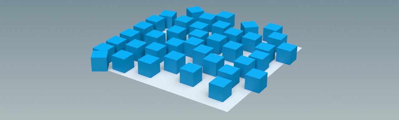
You’ll notice that several cubes have a rotation applied. This is because the points are relaxed. Relaxation means that the node tries to separate the instances to avoid overlapping. You can control the quality of this process with Relax Iterations. However, if the number of instances is too big, the separation process will fail anyway. To change the distribution of the cubes on the surface, try different Seed values.
Defining the instances by a number is a common method, but there are two more options on the Point Count Method dropdown:
-
Density can be seen as a “packing” rate and with higher values you’ll create more and densely packed instances
-
Face Centroid calculates the geometric center of a polygon and adds an instance to this point

Transforms tab 
The Transform tab provides parameters for randomizing orientation, rotation, and scale. The sections are expandable and contain more parameters.
The Surface Blend parameter aligns the up axis of the instances with the surface normals of the source object. A value of 1 means full alignment with the surface normal. With 0, the instances will be fully oriented along the up axis. With Variation, you can add some randomness to the orientation.
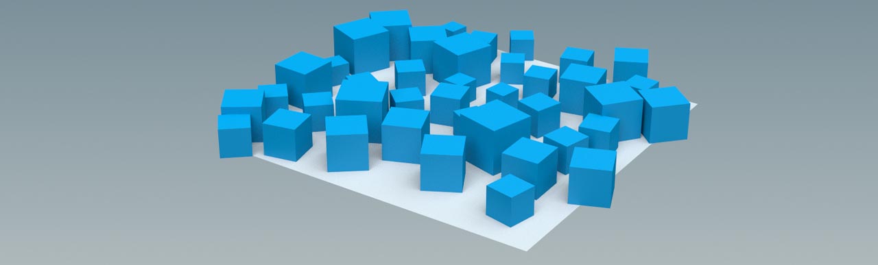
Now go to the Scale section. When you turn on Use Scale from Scatter and change Number of Instances, the node calculates a pscale attribute based on that very number. With an increasing number, the instances become smaller; with a decreasing number, the instances turn out bigger. This option effectively prevents overlapping objects. You can also define a global scale that is applied to all instances. With Variation, you’ll randomize the size of each instance.
The parameters for the rotation of the instances are located in the Spin section. The Spin parameter itself defines a global rotation, while Variation creates a random per-instance rotation.
Multiple prototypes 
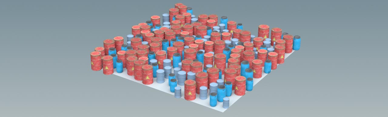
Most of the time you’ll use more than one prototype and simple geometry like boxes is also a rare case. To bring a scene to life, you typically have a set of assets. For city streets, you need lanterns, traffic lights, bins, manhole covers, all kinds of signs, roadblocks, trees, and so on.
When you work with multiple assets, you can chain or merge them on the stage. Please note that, if a SOP context contains merged assets, the output will be treated as one object. However, you can separate SOP-merged prototypes with proper naming by defining groups.
Prototype distribution 
If you've worked with different scatter techniques before, you might be missing a method that lets you control the distribution of the instances - aside from the Seed parameter. With points you can apply maps or noise to create clusters and zones of varying density. The Scatter Instancer LOP also provides this possibility, but the workflow is different.
When you expand the Scattering ▸ Number of Instances section, you can find two toggles:
-
Texture Map requires UVs and expects an image that will be mapped onto the source geometry
-
Primvar lets you define a point attribute on the source geometry
Textures 
You can load both grayscale and color maps. In the latter case, the node will use the map’s luminance for calculating the density values. Black areas have a density of 0 and are considered empty, white pixels represent maximum density.
Tip
On the Transforms tab, you can also use maps to drive the parameters of the Spin, Scale, and Position sections.

Primvars 
If you want to use a primvar to define the scatter density, you have to create a point attribute on the source geometry. Let’s say you have a basic grid inside a SOP context like the  SOP Create LOP and want to apply a
 density attribute.
To get a usable result, the number of points is of particular importance because the density values will be interpolated. If the distance between the point is too big, you’ll most probably not achieve good results. For a basic grid you can increase the Columns and Rows parameter, for example to 50. The higher the resolution of the source geometry, the better the result.
To create the density attribute, you can, for example, use the  Attribute Noise SOP and
  Attribute Paint SOP nodes. The paint node lets you precisely define areas with higher and lower density - even on a per-point basis.
Tip
On the Transform tab’s Spin section, you can use a vector Direction Primvar to introduce per-instance rotation values.
You can also achieve interesting result when you combine primvars with texture maps as in the image below. There, an Attribute Noise SOP was used to create the density attribute. The icon, on the other hand, controls the scale of the instances. In the white areas, scale is 0.

Masks 
Another, very efficient way to control the distribution of the scattered instances is masking. On the Scattering tab, there are five different methods, and you can combine these masks by turning them on and off. Masks are always applied to the source geometry.
Every mask type has an Invert option to flip the result.
Up Axis Direction 
The Scatter Instances LOP’s Up Axis parameter lets you choose which direction is considered “up” in your scene. By default, this is the positive Y axis. You can define an angle that specifies the maximum deviation from the up axis at which objects will be generated. Imagine you want to scatter rocks on a mountain. In areas with steep slopes, there shouldn’t be any rocks, because they would simply tumble down.
If you use a small Max Angle, you’ll only be accounting for areas with almost no slope. With bigger angles, you’ll cover more and more steep areas of the mountain. The number of instances remains constant even if the scatter area becomes smaller.
The Cast Shadows option sends out rays to mask areas that are occluded by an object, for example under a bridge.

Ambient Occlusion 
Occluded surface areas appear darker and you can use this behavior to create a mask. For example, if you don’t want plants to grow in corners or cervices. Other nearby meshes can also occlude certain parts of an object.
Only geometry within the Maximum Ray Distance contributes to the occlusion calculation. A small value means only very close geometry causes darkening. With large values, only distant geometry also contributes and creates broader, more global shadowing. The Input Min and Input Max parameters define, how far a ray can travel. When you increase the values, you get a higher probability that a ray hits an object. In the image, the values are 0.7 and 1.

Camera 
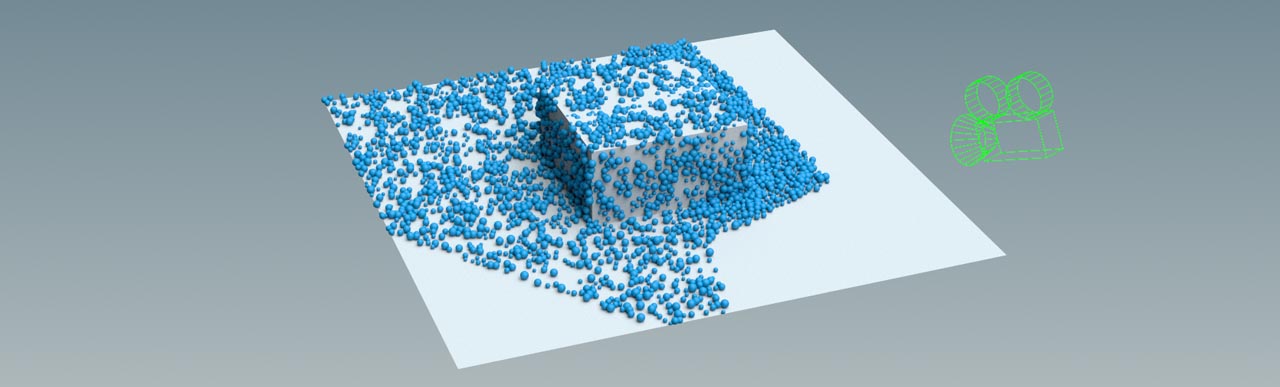
You can also use a camera to create a mask. To make this option work, you need to add a camera to the Camera Path parameter first. By default, all instances outside the camera frustum will be removed and you can control the accuracy of the mask with the Frustum Padding parameter. Negative values will narrow the frustum area, bigger values will make it wider.
You can use the Override Near Plane and Override Far Plane parameters to rearrange the camera’s focus planes and change the size of the actual scatter area.
PointInstancers 
You can use a point source, for example from another Scatter Instances LOP or a  PointInstancer LOP to create “seed” points. The actual scatterer will then add the instances around the seeds within the value of the Radius parameter. Falloff randomly removes instances to avoid hard edges. On the Prim Pattern parameter, you define the path to the source of the seed points.

Meshes 
You can also use meshes to create masks where everything inside the object(s) remains empty. On the Prim Pattern parameter you add the path to the mesh you want to use for the mask. Offset creates an empty area around the mesh, and Falloff adds “softness” to the masked area by randomly removing instances.
With Bounding Box Only, the scatter node won’t use the actual shape of the mesh for the creation of mask, but a box that completely encloses a piece of geometry.
Tip
If you don’t want to see the mesh that creates the mask, you can use a  Configure Primitive LOP. Add the mesh to the Primitives parameter and set Visibility to Invisible.

Prototypes 
The Prototypes tab lets you work on the base objects meant to be instanced. You can, for example, create groups or determine how the prototypes are finally chosen. The Method parameter’s dropdown offers three different ways how prototypes are combined.
By default, you’ll connect the prototypes to the Scatter Instances LOP’s second input. The parameters under Copy Prototypes from Second Input manage the handling of the incoming objects. The Destination ▸ Root Prim parameter let’s you define, where in the Scene Graph Tree, the instances will appear.
The default entry is composed from the Scatter Instances LOP’s Primitive Path parameter and /pointinstancer/Prototypes.
You can also find this path on the Prototype Group 0 ▸ Prim Pattern parameter, but there it’s terminated with a * wildcard. This means that all primitives that live under this path, will be added to Group 0.
Groups and patterns 
You can create new groups by increasing Prototype Groups. Each group will have its own parameter set and you can add primitives by specifying a Prim Pattern. Prim patterns are regular expressions that let you combine or exclude primitives. For example, you have five assets named asset_1 -> asset_5, but you only want to consider number 1, 3, and 5. In such a case, the pattern would be asset_[135].
Weights 
This is the Method parameter’s default option and adds a Weight parameter to each prototype group. Weight controls, how often a prototype will finally be instanced. Note that the sum of all Weight values can be smaller or greater than 1. With Reset All Weights, the parameters will be set to a value of 1.
Even when all Weight parameters are set to 1, it is possible for one object to outnumber the others. This is because the node has an internal distribution mechanism. For example, with two objects, 100 instances and Weight parameters of 1, the resulting ratio is not necessarily 50:50.

Texture Map 
The Method dropdown menu’s second option expects a texture file. The map’s integers correspond with the number of prototype groups. You can, for example, create such a texture in Copernicus. Please note that there’s currently no live link to Houdini’s Copernicus framework and you have to save the image to disk. Then, load the file to the Texture Map parameter.
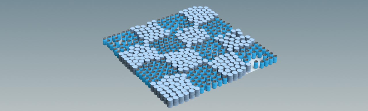
Primvar 
You can also author a protoid point attribute to the source geometry. The attribute’s values can be an integer or a float that represents the prototype groups, for example 0 to 2 if you have three groups defined. The method is the same as described in the Primvar chapter above. The difference is that the attribute is valid for complete groups instead of individual prototypes.
On the Primvar parameter, enter the name of the attribute.

Shading 
The Scatter Instances LOP’s Shading tab lets you author custom primvars for randomizing certain aspects of a MtlX shader. Furthermore, the node also creates several primvar you can read and apply directly to a material definition. This can be a Quick Surface Material or a MtlX material inside a  Material Library LOP.
Random colors 
A typical application is the creation of random colors. If you want to change the base color of a Quick Surface Material, go to the material’s Base ▸ Color Primvar and enter the name of the primvar, for example randomColor.
To make the instancer aware of this primvar, open its Shader tab and set Random Primvars to 1. This creates a new parameter set with a Name parameter. There, enter randomColor. Then, change Type to Color (RGB) and define the min and max values for the primaries.

When you take a closer look at the quick material’s various sections, you can see several more placeholders for primvars. Please remember that material properties like roughness or emission are floats, not color vectors.
If you want to work with a Karma material inside a Material Library LOP, you can use the  MtlX Geometry Property Value VOP to read out the
 randomColor primvar. Then, connect the property node to the appropriate input of the MtlX Standard Surface VOP. The MtlX OpenPBR Surface VOP is also supported.
Scatter primvars 
The Scatter Instances LOP authors several primvars and you can see them when you click the pointinstancer primitive in the Scene Graph Tree. The primvars are listed in the Scene Graph Detail pane’s Name column. The entries of interest start with a primvars: prefix and have float or int signatures. Primvars with three floats inside squared brackets are interpreted as vector3 or color.
You can use the built-in primvars without going a detour via the Point Instancer LOP. Instead, you use the name of attribute directly with the Quick Material Surface or the MtlX Geometry Property Value VOP, for example protoid. Note that, with the geometry property node, you also have to choose the correct Signature. The image shows the visualization of the protoid primvar.

Animated source geometry 
Note
The support for animated source geometry is in beta state because motion blur is currently not supported.
You can also use animated geometry for the Scatter Instances LOP’s Source Geometry ▸ Prim Pattern parameter. Then, from the Animation (Beta) dropdown menu choose Deforming Transforms. If the surface is just transforming, not deforming, choose Rigid Transforms.
If you source geometry has a rest attribute, add it Input Primvars ▸ Rest Primvar.
Alternative workflow 
The previous examples and chapters have assumed that all prototypes are connected to the Scatter Instances LOP’s second input. However, there’s also a workflow with prototypes available at the first input. This method can speed up the scattering process, but requires a few small changes to the workflow.
Prototype visibility 
When you connect prototypes to the first input, you typically want to hide them because they’ll be rendered with the instances. For this purpose, you can add a Configure Primitive LOP upstream of the Scatter Instances LOP:
-
Use Primitives to define the prototype(s) you want to hide
-
From the Visibility dropdown, choose Invisible
-
Expand the Schema section and set Type to Scope
-
Turn on Primitive Specifier
Tip
It can happen that a prototype is being rendered in the viewport although it has been made invisible. In this case, restart the render.
Prototype groups 
To make the instancer aware of the prototypes, you need groups. You can combine all primitives in a single Prototype Group or create individual groups for every prototype. Alternatively, you can also apply prim patterns to manage your selections. Having one group per prototype or pattern lets you make use of the Weight parameter.
