| On this page |
|

Overview 
In the KineFX rigging and animation framework, a character’s skeleton is represented at the geometry level by a collection of points connected by polygon lines. This joint-based system allows the character’s joint hierarchy to be created and edited using SOP nodes, and from this, we are able to procedurally build characters by creating and manipulating the character’s skeleton and skin. This character is then piped into rig logic, which determines how the character rig behaves.
Pre-Houdini 20, a character’s rig logic lived in rig behavior nodes (like the ![]() Rig Pose SOP) and was also evaluated on those nodes. This meant that once we came to the point in the network that determined how a rig behaved, this functionality had to be evaluated at that exact place in the network, i.e. the rig logic and rig evaluation were tied together in the same place in the network.
Rig Pose SOP) and was also evaluated on those nodes. This meant that once we came to the point in the network that determined how a rig behaved, this functionality had to be evaluated at that exact place in the network, i.e. the rig logic and rig evaluation were tied together in the same place in the network.
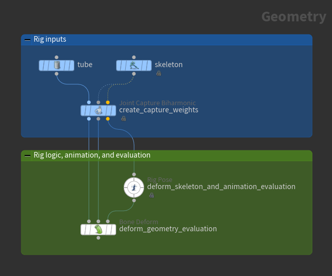
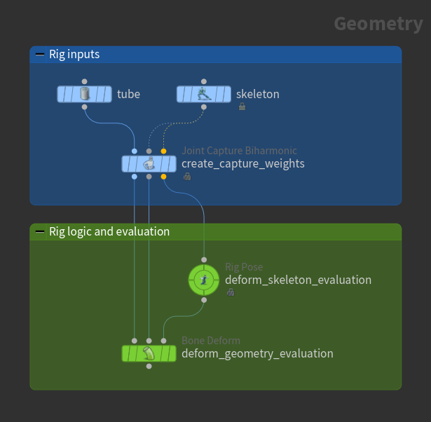
In the example below, we have a simple pre-Houdini 20 rigging setup where a tube geometry is being deformed. The inputs to the rig are set up by creating the tube geometry, the skeleton, and the capture weights on the geometry. On the ![]() Rig Pose SOP, the pose of the skeleton can be manipulated (the skeleton is deformed), and animation can be added by setting keyframes. The Rig Pose SOP then evaluates the skeleton deformation and animation, and the result of this evaluation is piped into the
Rig Pose SOP, the pose of the skeleton can be manipulated (the skeleton is deformed), and animation can be added by setting keyframes. The Rig Pose SOP then evaluates the skeleton deformation and animation, and the result of this evaluation is piped into the ![]() Bone Deform SOP, where another evaluation is performed and the geometry is deformed.
Bone Deform SOP, where another evaluation is performed and the geometry is deformed.
There are a few issues with this approach:
-
To deform the geometry on a skeleton, there are two evaluation steps - one on the Rig Pose SOP and the other on the Bone Deform SOP, and there is an evaluation dependency between the two.
-
The rig logic and rig evaluation are tied together. Whenever you change the pose of the skeleton on the Rig Pose SOP, this change is evaluated.
-
The animation (on the Rig Pose SOP) and the deformed result (on the Bone Deform SOP) must be viewed on different nodes.
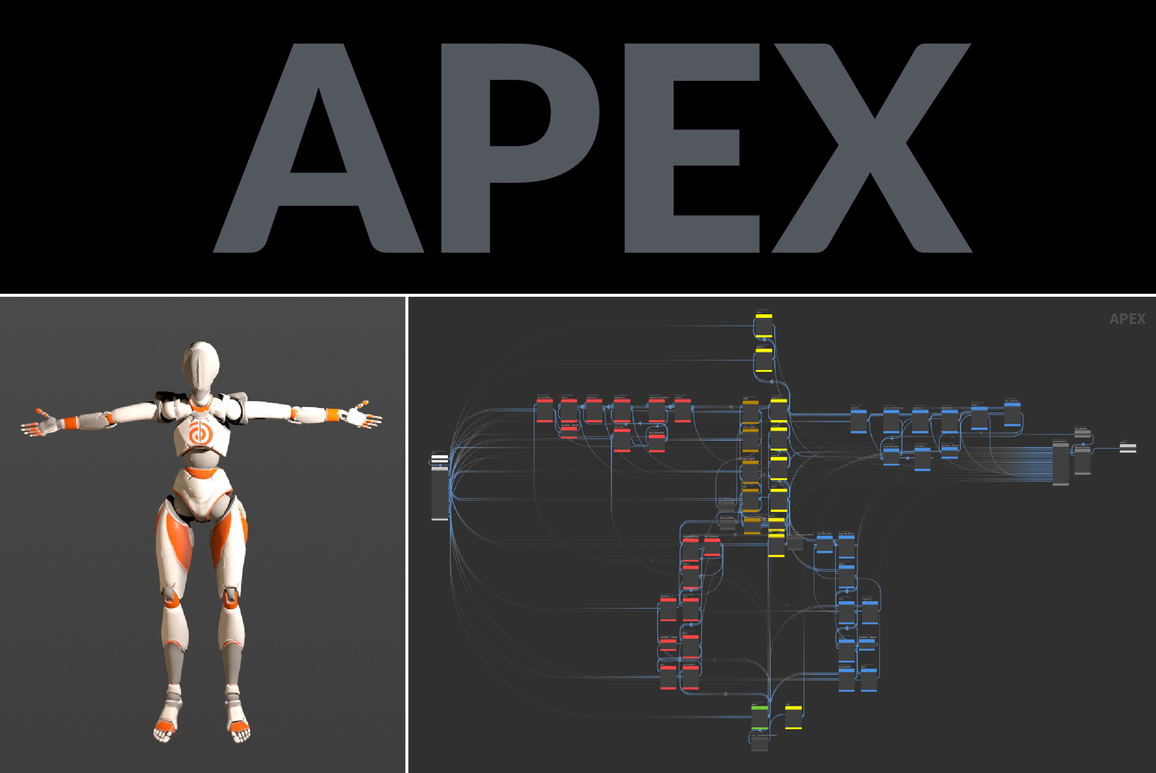
APEX (All-Purpose EXecution) 
With Houdini 20, we introduce APEX (All-Purpose EXecution), Houdini’s new graph evaluation framework that builds and runs graphs, and fetches their results. Within the KineFX rigging framework, APEX graphs are used to represent the rig logic.
In APEX, a graph is a piece of logic that, when evaluated, performs a specific task. APEX graphs can also be built up to perform more complex functionality like determining how an entire character behaves, complete with an FK hierarchy for the skeleton, and logic to deform geometry.
In rigging with APEX, we still have the same steps for assembling and preparing the input elements to deform - creating the geometry, the skeleton, and the capture weights on the geometry - but APEX graphs are now used as the rig logic representation.
|
Pre-Houdini 20 |
Houdini 20 |
|
|---|---|---|
| Assembling and preparing rig inputs | Build a skeleton and create capture weights | Same as pre-Houdini 20 |
| Rig logic |
Rig behavior nodes
(for example, |
APEX graphs |
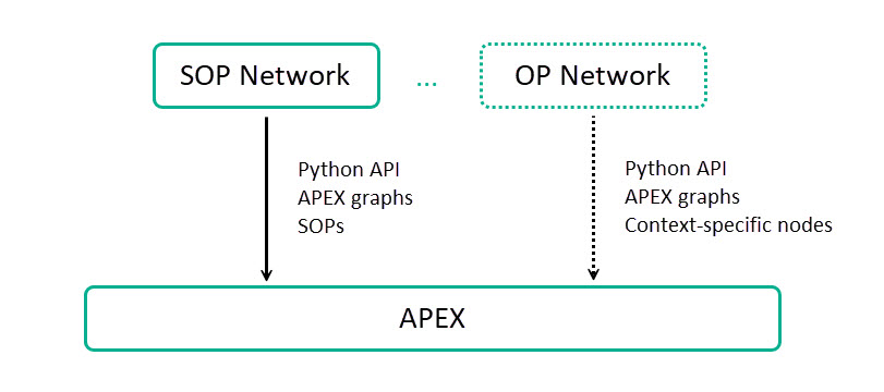
APEX sits at a layer below SOPs and is not tied to any network context. You can build, manipulate, and run APEX graphs using the Python API, other APEX graphs, and SOPs. In the future, there may be other contexts that can access and utilize APEX graphs.
Note
For users who are familiar with VOPs and VEX, APEX is a mid-level visual programming framework - higher than VEX and lower than SOPs. In VOPs, we are limited to the types that VEX understands. APEX is essentially procedural VOPs with support for more types (via an extensible type system).
Delayed evaluation 
In the SOP context, APEX graphs are a piece of geometry. The rig logic represented by an APEX graph is built up in the SOP network as the graph is passed from SOP node to SOP node, with pieces of logic added to or changed on the graph along the way. When building of the graph is complete, the rig logic is evaluated at a point in the network of your choosing (using the APEX Invoke Graph SOP or ![]() Python SOP), or through a specific action in the viewport.
Python SOP), or through a specific action in the viewport.
This idea of delayed evaluation of the rig logic allows you to procedurally build up rig logic pieces and assemble them together without having the rig constantly evaluating and calculating, which significantly impacts performance. Delayed evaluation also allows you to choose when and where the rig logic is evaluated, instead of having the evaluation performed whenever you visit a rig behavior node like the Rig Pose SOP. In APEX, evaluation of the graph is always delayed - you build up the graph logic, and choose to evaluate the graph at a later point in the network.
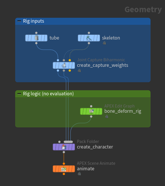
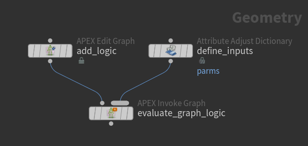
In the APEX workflow example below, all of the rig logic lives in the ![]() APEX Edit Graph SOP,
APEX Edit Graph SOP, bone_deform_rig. The rig logic is not evaluated in any part of the network, so there is a clear delineation between the rig setup steps (assembling the rig inputs and defining the rig logic) and the rig evaluation.
Rigging in APEX 
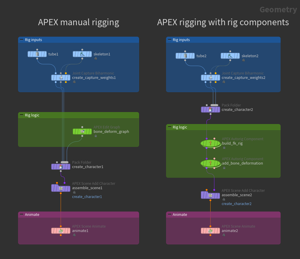
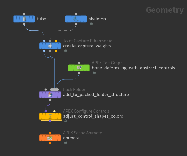
In the APEX rigging workflow, you can build up the rig logic by either manually creating a graph or using rig components. In the example below, the purple nodes build up the rig logic, create the characters, and assemble the scenes in preparation for animation.
See the packed character format and the animation workflow for information on creating characters and assembling animation scenes.
Graph building 
APEX graphs take in data in the form of input parameters, perform operations on the data, and make data available to be fetched as outputs. Within a graph, geometry can be manipulated alongside other types, so you can, for example, perform numerical and matrix operations on skeleton joint transforms all in one graph.
Note
The type of data that APEX graphs can output is limited only by the context within which the graph is run. When run in SOPs, graphs can output geometry, as well as any data that can be stored in a dictionary attribute on the geometry. When run in Python, graphs can output the types that can be cast to a Python type.
The APEX network view is used to visualize and build graphs, and it can write directly to the ![]() APEX Edit Graph SOP. To start building a graph:
APEX Edit Graph SOP. To start building a graph:
-
At the geometry level, create an APEX Edit Graph SOP in the network editor.
-
With the APEX Edit Graph SOP selected, click the
 New Tab icon at the top of the pane where you want to open the APEX network view, and select New Pane Tab Type ▸ Animation ▸ APEX Network View.
The APEX network view shows the graph that is stored on the APEX Edit Graph SOP.
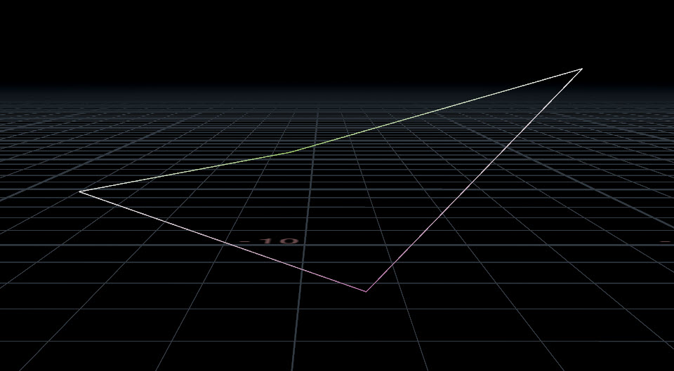
The graph structure is represented as geometry, where the nodes in the graph are represented as points in the viewport, and the connections between the nodes are represented as lines between these points. In the example below, the positions and colors of the graph nodes and and their connections directly correlate to the points and edges in the viewport.
When the position and color of the graph nodes change, this is reflected in the geometry in the viewport.
The components of the graph and geometry have the following correlation:
Graph (visualized in the APEX network view) |
Geometry (visualized in the viewport) |
|---|---|
|
Points |
|
Wires |
Line primitives |
Input and output ports on connected nodes |
Vertices |
Input parameters on the |
Parameters stored on the geometry |
Graph nodes, subgraphs, and subnets 
Graph nodes perform a specific operation and can be APEX functions, verbs, subgraphs, or subnets.
APEX functions
APEX functions perform a specific operation on whatever is connected to its input ports.
Verbs
A verb is the basic operation of an OP node. It does not include other operations that relate to the node like caching, reading inputs, and evaluating parameters. For example, the ![]() Joint Deform SOP is an HDA wrapper around the bonedeform verb, so Joint Deform cannot be used in APEX graphs, but bonedeform can.
Joint Deform SOP is an HDA wrapper around the bonedeform verb, so Joint Deform cannot be used in APEX graphs, but bonedeform can.
Subgraph
A subgraph is a locked graph and is similar to an HDA in that modifying a subgraph modifies all instances of the subgraph. The SmoothIK node is an example of a subgraph.
Subgraphs are stored as a subgraph library in a .bgeo geometry file. A subgraph library has the following structure:
-
A single unpacked APEX graph, where the subgraph name is defined by the
namedetail attribute.or
-
A number of packed geometry primitives, each containing an APEX graph. For each of the primitives, the subgraph name is defined by the top-level
nameprimitive attribute.
The subgraph .bgeo files are loaded from the @/apexgraph directories, where @ expands to the directories in the HOUDINI_PATH.
Subnet
A subnet is a container that encapsulates multiple graph nodes inside a single node. This simplifies and improves the readability of the graph containing the subnet. If you create several subnets with the same contents, updating one of the subnets will not affect the others.
| To... | Do this |
|---|---|
|
Save an unpacked graph to a subgraph library file |
When saving an unpacked APEX graph to a subgraph library file, a 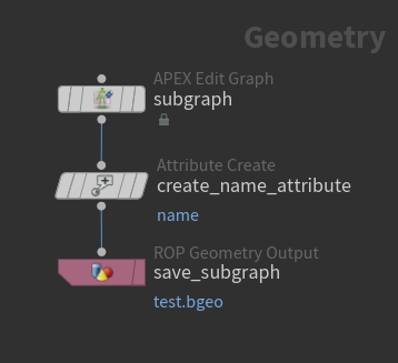
To load the saved subgraph:
|
|
Save packed graphs to a subgraph library file |
Use a 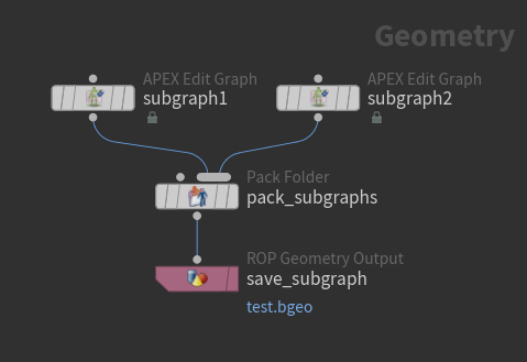
To load the saved subgraphs:
|
|
Update all subgraph instances |
After making changes to a subgraph, update all the subgraph instances by doing the following:
|
|
Create a subnet |
|
|
Change the port name of a subnet |
Dive into the subnet and change the port name on the Note Only subports can be renamed. “Regular” ports cannot be renamed. Subports are created when connections are made to variadic ports. See ports for more information. |
Ports 
You can connect nodes together in the APEX network view by creating wires between the ports on the nodes. Port values come from either port connections, the values set in the node parameter window, or certain default values.
The node parameter window is used for editing the port’s values. To bring up the node parameter window, select a graph node and press P.
Port |
Value |
|---|---|
Connected ports |
Values from connections override the values set inside the node parameter window. |
Unconnected ports |
Unconnected port values come from either the values set in the node parameter window, the corresponding SOP verb nodes, or default values set internally in APEX. 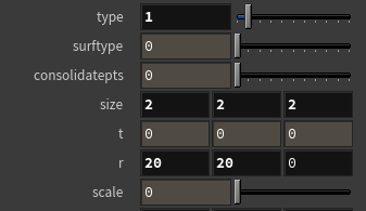
Ports that appear in the node parameter window with a black background are present in the geometry spreadsheet
Ports that appear in the node parameter window with a gray background are not present in the
Note The values displayed in the node parameter window are not always the values used by the ports. If a port is not present in the geometry spreadsheet |
Different port colors refer to different data types on the port. There are also two special types of ports - variadic ports and in-place ports:
Variadic port
You can make multiple connections to a variadic port, and subports are created on the node. The port next is an example of a variadic port that exists on several nodes. There are also other variadic ports on specific nodes, for example, the b port on the Add node, and the transforms port on the GetPointTransforms and SetPointTransforms nodes.
Note
Only subports can be renamed. “Regular” ports cannot be renamed. Rename subports by ![]() clicking the subport name.
clicking the subport name.
In-place port
The value of in-place ports are updated without creating a copy. In-place ports are identified with a square.
Basic graph operations 
The examples in this section follow the basic structure of:
-
How to create the graph logic.
-
How to evaluate (execute) the graph.
The examples in this file demonstrate how to create APEX graphs that perform the basic graph operations in this section.
Add two values 
This example shows how to create a graph that adds two values. We will go through the basic workflow of how data is input into the graph and how to view the output of the graph.
Create the graph logic 
Create the logic to add two values, a and b.
-
At the geometry level, create an
 APEX Edit Graph SOP in the network editor.
 -
With the APEX Edit Graph SOP selected, open the APEX network view. The APEX network view can write directly to the APEX Edit Graph SOP.
-
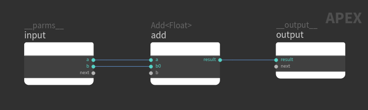
In the APEX network view, create a graph that performs a simple numerical operation:
-
Add the graph input and output nodes:
-
Add the node that takes in the input parameters. Press TAB to bring up the TAB menu and search for Input. The
inputnode will be added to the graph. -
Add the graph output node by searching for Output in the TAB menu.
-
-
Add an Add<Float> node to perform a simple add operation.
-
Connect the nodes as follows:
On the
addnode, b is a variadic port, so you can make multiple connections to it, and subports named b<x> will be created.Connect the nodes in the APEX network view
-
At this point, the inputs of the graph have not been defined and the graph is not being evaluated or calculated, so there is no output or result. The graph is only a piece of logic represented as geometry.
Define the inputs 
We now define the inputs, a and b, of the addition operation. Numerical inputs must be stored in a dictionary format, and so the dictionary is essentially a container of our input data. A dictionary stores a set of key/value pairs, and in our case, a and b are the keys. We use an ![]() Attribute Adjust Dictionary SOP to create a dictionary for the input parameters.
Attribute Adjust Dictionary SOP to create a dictionary for the input parameters.
In the Attribute Adjust Dictionary SOP, set the values for a and b:
-
In the Set Values section, create two entries by clicking
 beside Number of Entries.
 -
For the 1st entry, set the following:
-
Key:
a -
Type: Float (we are adding float values)
-
Value: Assign a value to
a.
-
-
For the 2nd entry, set the following:
-
Key:
b -
Type: Float
-
Value: Assign a value to
b.
-
By default, Attribute Name is set to parms, and Attribute Class is set to Detail, so we have a detail attribute called parms. This new parms attribute can be viewed in the geometry spreadsheet:
-
At the top of the pane where you want to open the geometry spreadsheet, click the
New Tab icon and select New Pane Tab Type ▸ Inspectors ▸ Geometry Spreadsheet. -
Select
 Detail from the top toolbar.
Evaluate the graph logic 
We have now defined the graph logic as well as the graph inputs. To invoke (or evaluate) the graph, use the APEX Invoke Graph SOP.
-
Connect the node network:
-
The 1st input of the APEX Invoke Graph SOP takes in an APEX graph. In the network editor, connect the APEX Edit Graph SOP (contains the graph) to the APEX Invoke Graph SOP (1st input).
-
The 2nd input of the APEX Invoke Graph SOP takes in the data we want to use as inputs. They could be numerical values in a dictionary format, or regular geometry. Connect the Attribute Adjust Dictionary SOP to the APEX Invoke Graph SOP (2nd input).
Add two numerical values using a graph -
-
Specify the inputs in the APEX Invoke Graph SOP:
-
Add an input by clicking
beside Input Bindings. -
By default, Dictionary To Bind is turned on and set to
parms. This is what we want because earlier, we had used the Attribute Adjust Dictionary SOP to define our input as a dictionary calledparms.
-
-
Specify the outputs to fetch in the APEX Invoke Graph SOP:
In this case, we are fetching numerical values (not geometry), so specify an output to fetch by clicking
beside Output Dictionary Bindings. The output is stored in a dictionary format.-
Apex Outputs Group is the name of the output node in the graph. In our case, it is
output. -
Set Output Attrib to a name for the output dictionary, for example,
output_parms.
-
The new output_parms dictionary holds the calculated results. It can be viewed on the geometry spreadsheet by selecting ![]() Detail from the top toolbar. The
Detail from the top toolbar. The output_parms dictionary has the key result (the name of the port on the graph output node) set to the value a + b.
The APEX Invoke Graph SOP evaluates (calculates) the logic from the APEX graph and gives you the result. If you change the values of a and/or b in the Attribute Adjust Dictionary SOP, the output dictionary calculated by APEX Invoke Graph is updated to the new sum.
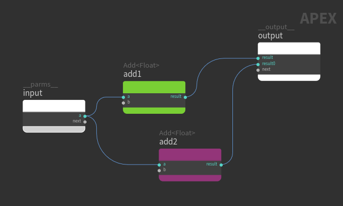
Fetch two results 
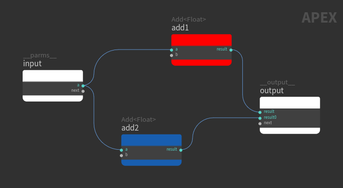
We now take the graph logic from the previous example, perform another operation on the original result, and fetch the two results.
Create the graph logic 
Starting with the previous graph, add a node that divides the result of the previous sum. Then output the result of the divide operation.
-
In the APEX network view, add a Divide<Float> node (red node is new). The subports on the
divideandoutputnodes have been renamed. The b port on thedividenode is a variadic input.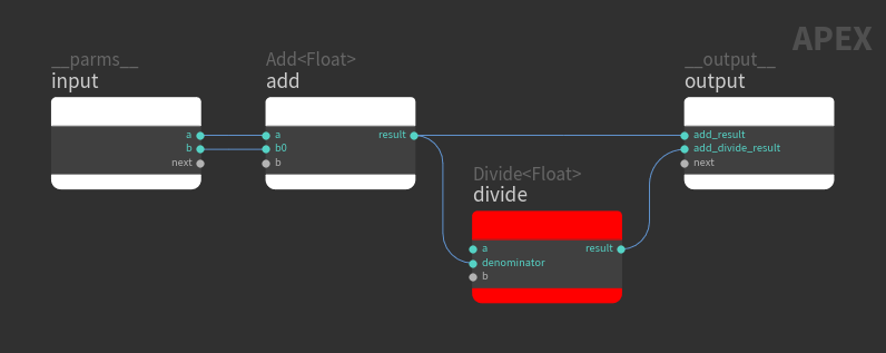
Graph logic that outputs two results There are now two values on the
outputnode. -
Set the values on the
dividenode.-
Select the
dividenode and press P to bring up the node parameter window. -
divideperforms the operation a divided by b. In the node parameter window, set the value of a to, say,1.0. The value of denominator comes from the previous addition operation.
-
Evaluate the graph logic 
The graph inputs remain the same, so nothing needs to change in the Attribute Adjust Dictionary SOP.
For the graph outputs, the APEX Invoke Graph SOP is still fetching from the graph output node as it was doing previously. The difference now is that instead of getting just one result (the sum of the two inputs in add_result), we are also getting a second result (the outcome of the divide operation in add_divide_result). In SOPs, both results end up in one dictionary.
On the geometry speadsheet, view the values that are fetched from the graph output node:
-
Select the APEX Invoke Graph SOP in the network editor.
-
In the geometry spreadsheet, select
Detail from the top toolbar. -
The following two values are fetched from the
outputnode:-
add_result: Sum of graph inputs a and b.
-
add_divide_result: <
dividenode port a> / <sum of graph inputs a and b>
-
Note
The output dictionary contains all the results on the graph output node specified in the APEX Invoke Graph SOP parameter Apex Outputs Group.
Partial evaluation 
In this example, we introduce the idea of partial evaluation, where we only get the outputs that we ask for, and only those outputs are being calculated, with the rest of the graph logic being ignored.
Create the graph logic 
Start with the add-divide graph from the previous example. Add another output node and give it a different name from the original output node.
-
Add a second output node and rename it to, say,
output2. -
Add a Multiply<Float> node.
-
Connect the nodes as follows (red nodes are new in this example):
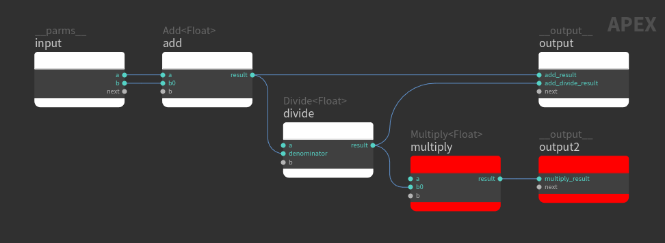
Partial evaluation of graph logic -
Set the values in the
multiplynode.-
Select the
multiplynode and press P to bring up the node parameter window. -
In the node parameter window, set the value of a to, say,
2.0. The value of b0 comes from the previous divide operation.
-
Evaluate the graph logic 
View the values that are being fetched:
-
Select the APEX Invoke Graph SOP in the network editor.
-
In the geometry spreadsheet, select
Detail from the top toolbar.
As in the previous example, the same output_parms dictionary from the original output node is being fetched (the values fetched are add_result and add_divide_result). Even though we've specified another output node, only the values that we are asking for in the APEX Invoke Graph SOP are being fetched.
Note
In this case, partial evaluation is performed on the graph logic. Only the logic that calculates the values in the output node is exercised because we are only asking for the values in output. The logic that calculates the values in output2 is ignored.
To also fetch the values from the new output node, output2:
-
In the APEX Invoke Graph SOP, click
beside Output Dictionary Bindings to add another output node to fetch from. -
In the new Output Dictionary Bindings entry:
-
Set Apex Outputs Group to
output2. You could also selectoutput2from the drop down box. -
Set Output Attrib to a name for the output dictionary, for example,
output2_parms.
-
View the values that are now being fetched:
-
Select the APEX Invoke Graph SOP in the network editor.
-
In the geometry spreadsheet, select
Detail from the top toolbar.
The values from the two output nodes, output and output2, are now being calculated, fetched, and stored in two dictionaries, output_parms and output2_parms.
Modify geometry based on a numerical operation 
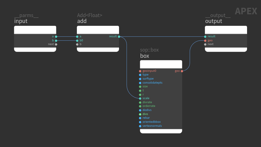
This example shows how to modify the size of a box geometry based on the result of an add operation.
Create the graph logic 
-
Start with a graph that adds two numbers.
Graph logic that adds two numbers -
Add a box geometry, the
 sop::box node. The result of the add operation is connected to the scale of the box geometry, so the sum of the add operation affects the size of the box.
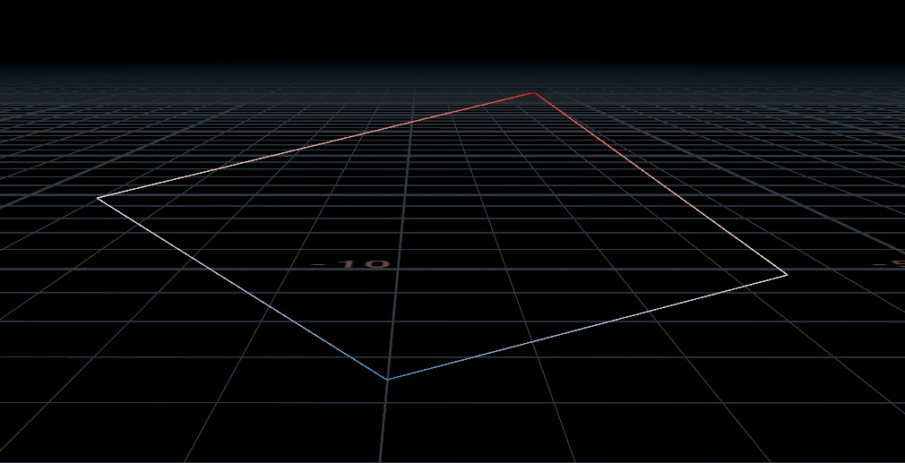
Numerical operation affects the size of box geometry
Evaluate the graph logic 
This time, we want to fetch geometry instead of just numerical values. To view the box, we need to fetch the box geometry on the output node:
-
In the APEX Invoke Graph SOP, turn on Bind Output Geometry and set its value to
output:geo(<name of output node>:<geometry on output node>). -
Set the display flag on the APEX Invoke Graph SOP. You can see the box in the viewport.
Select the Attribute Adjust Dictionary SOP to see the graph input parameters,
aandb, in the parameter editor, but keep the display flag on the APEX Invoke Graph SOP. If you adjust the values ofaandbon the Attribute Adjust Dictionary SOP, the size of the box will change in the viewport.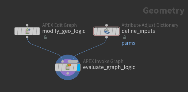
Network to adjust the input parameters and view the geometry
Retrieve and use information from geometry 
We can retrieve information from a piece of geometry to perform additional operations using that information. In this example, we place a sphere at one corner of a box geometry, and as we change the input parameters, the size of the box and sphere both change.
Create the graph logic 
-
Start with the box geometry graph from the previous example.
-
Add the red nodes below. In this graph logic, the sphere is placed at a specified corner of the box geometry, and the sphere and box are merged as one geometry to output.
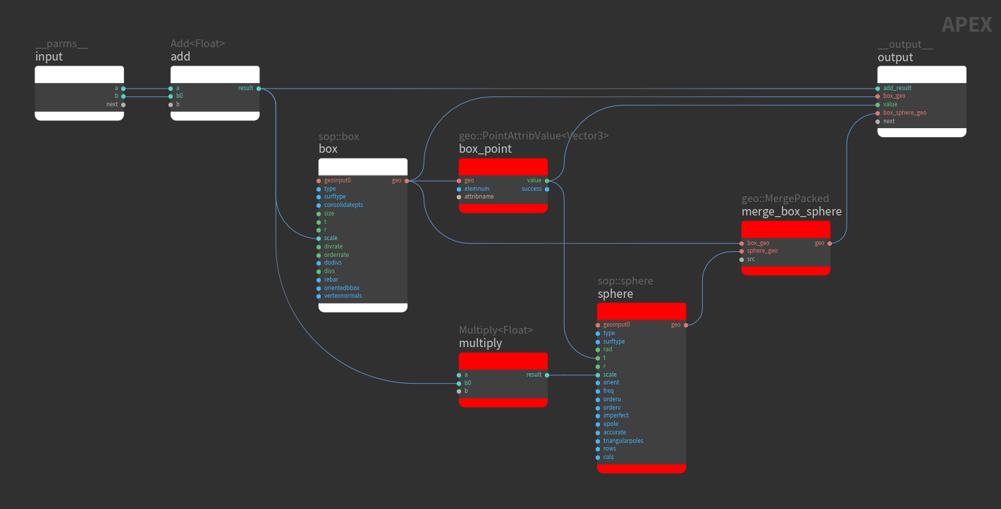
Retrieve information from a box geometry to perform additional operations
Node |
Description |
|---|---|
|
The To set the point location:
|
|
The To set the value of a, select the |
|
The box and sphere are merged as one geometry by connecting the geo outputs of The output of |
Evaluate the graph logic 
To view the box and sphere together, we need to fetch the merged box and sphere geometries on the output node:
-
In the APEX Invoke Graph SOP, turn on Bind Output Geometry and set its value to
output:box_sphere_geo(<name of output node>:<merged geometry on output node>). -
Set the display flag on the APEX Invoke Graph SOP to see the box and sphere in the viewport.
Select the Attribute Adjust Dictionary SOP to see the graph input parameters,
aandb, in the parameter editor, but keep the display flag on the APEX Invoke Graph SOP. If you adjust the values ofaandbon the Attribute Adjust Dictionary SOP, the size of the box and sphere will change in the viewport.Sphere stays at a point on the box
Graphs for the animate state 
The animate state is a new viewer state that can display multiple characters in a scene and allow users to perform posing such as FK or IK for characters, interact with controls on characters, and create constraints between characters. The animate state interprets an APEX graph, evaluates the graph, and displays the evaluated output in the viewport.
To build a graph for evaluation in the animate state, certain conventions need to be followed in addition to the regular graph building methods. In this section, we present some examples of how to build graph logic for specific functionality used in the animate state, such as creating controls and constraints, defining joint hierarchies, and performing geometry deformations.
Note
We will use the term rig or rig graph to refer to a graph that has controls and geometry that an animator can interact with in the animate state. The term graph is more generic and can have purposes beyond an interaction element in the animate state.
An important point to note is that only packed character elements can be displayed in the animate state. Once you finish building up a rig graph, the rig graph needs to be added to a packed folder structure in order for it to be picked up and displayed in the animate state. See the packed character format for information on how to prepare character data for evaluation in the animate state.
The examples in this file demonstrate how to use APEX graphs to build functionality for the animate state.
Controls 
A control is something that the user can interact with in the animate state. In this example, we introduce a special APEX node, TransformObject. TransformObject manages the transform behavior of elements, including defining transform hierarchies between elements. It also handles animation-friendly transform component inputs like translation, rotation, and scale, with a defined rotation order. When a TransformObject node is put in a graph, and its parameters are promoted (connected to the graph’s input node), the TransformObject element is picked up by the animate state and turned into a control - it is displayed as something the user can interact with.
Create the rig logic 
-
At the geometry level, create an
APEX Edit Graph SOP in the network editor. -
With the APEX Edit Graph SOP selected, open the APEX network view. The APEX network view can write directly to the APEX Edit Graph SOP.
-
In the Apex network view, create a graph that adds a control for a geometry.
-
Add the graph input and output nodes:
-
Add the node that takes in the input parameters. Press TAB to bring up the TAB menu and search for Input. The
inputnode will be added to the graph. -
Add the graph output node by searching for Output in the TAB menu.
-
-
Add the nodes that move the geometry around:
Node
Description
torusThe torus geometry to move around.
TransformObjectDefines and manages hierarchical transform behavior. To be able to manipulate transforms in the animate state, you need to promote the desired input parameters on the TransformObject node by connecting the parameters to the
inputnode. Once you promote a parameter on a TransformObject node, that TransformObject element is turned into a control that the user can interact with in the animate state.In this example, the translate (t) and rotate (r) parameters are promoted, so the user has access to the translate and rotate components of the control in the animate state.
transform_geoChanges the position of the torus.
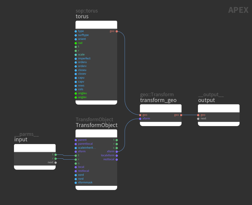
Rig logic to move a geometry using a control
-
Evaluate the rig logic using the animate state 
In the viewport, the graph itself is represented as geometry:
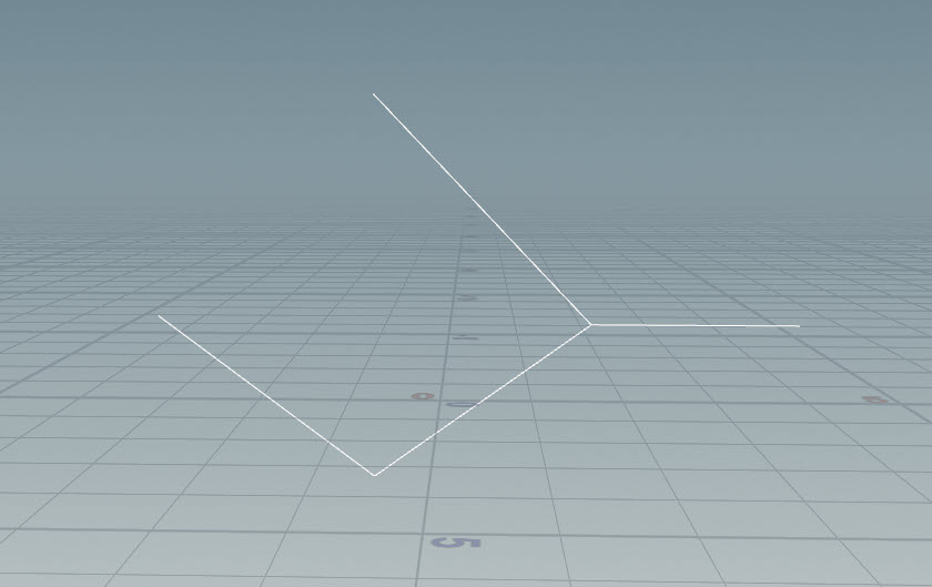
To see the output of the graph, you need to enter the animate state. The animate state automatically interprets the graph and displays the evaluated output. The animate state also creates controls for all the promoted parameters (in our case, the translate and rotate parameters) and allows you to interact with these controls.
To enter the animate state:
-
Connect the node network as follows.
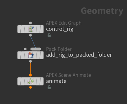
Network to enter animate state The
 Pack Folder SOP packs the rig into a packed folder structure. Only packed character elements can be displayed in the animate state.
 -
On the Pack Folder SOP, the Name parameter is automatically populated when an input is connected to the SOP. Specify the Type of the input as
rig.rigis a special extension that tells the animate state that the input contains the rig logic. -
Select the
 APEX Scene Animate SOP, and click
  Animate on the left toolbar or press Enter in the viewport.
In the video below, we are in the animate state. The white dot in the middle of the torus is the control. When the control is clicked, the translation and rotation handles are displayed because those parameters are promoted.
When you interact with controls in the animate state, the promoted parameters are modified, and these parameters are used as inputs to the graph logic. Every time you drag a control, the graph is evaluated with the updated parameters.
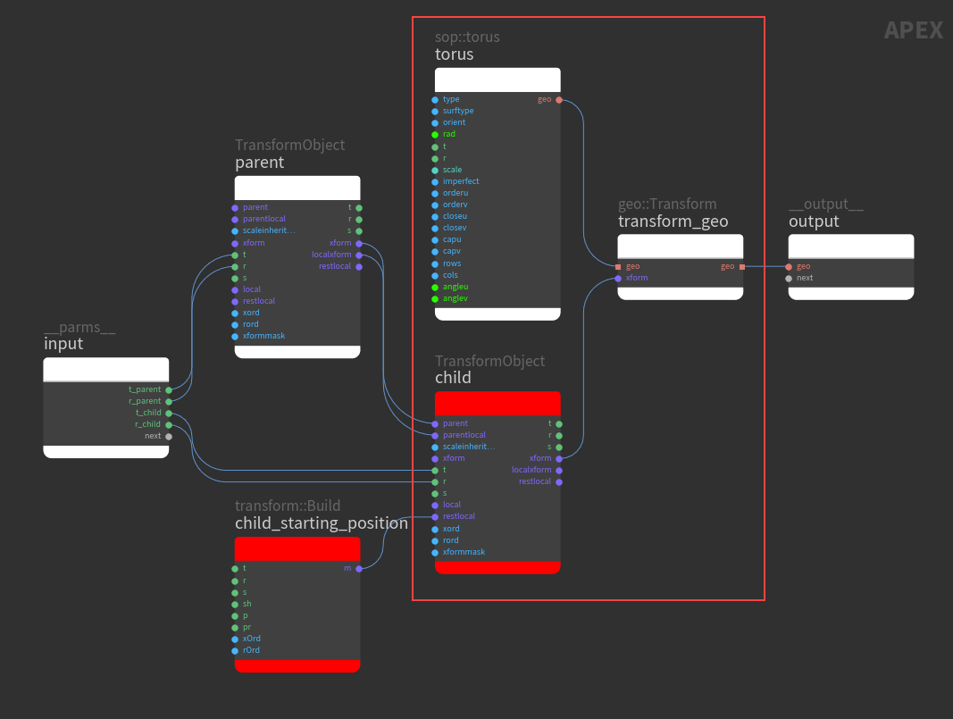
Parent-child hierarchy 
In this example, we create a parent-child node hierarchy.
Create the rig logic 
-
Start with the torus control rig from the previous example.
-
Add a child control (red nodes are new):
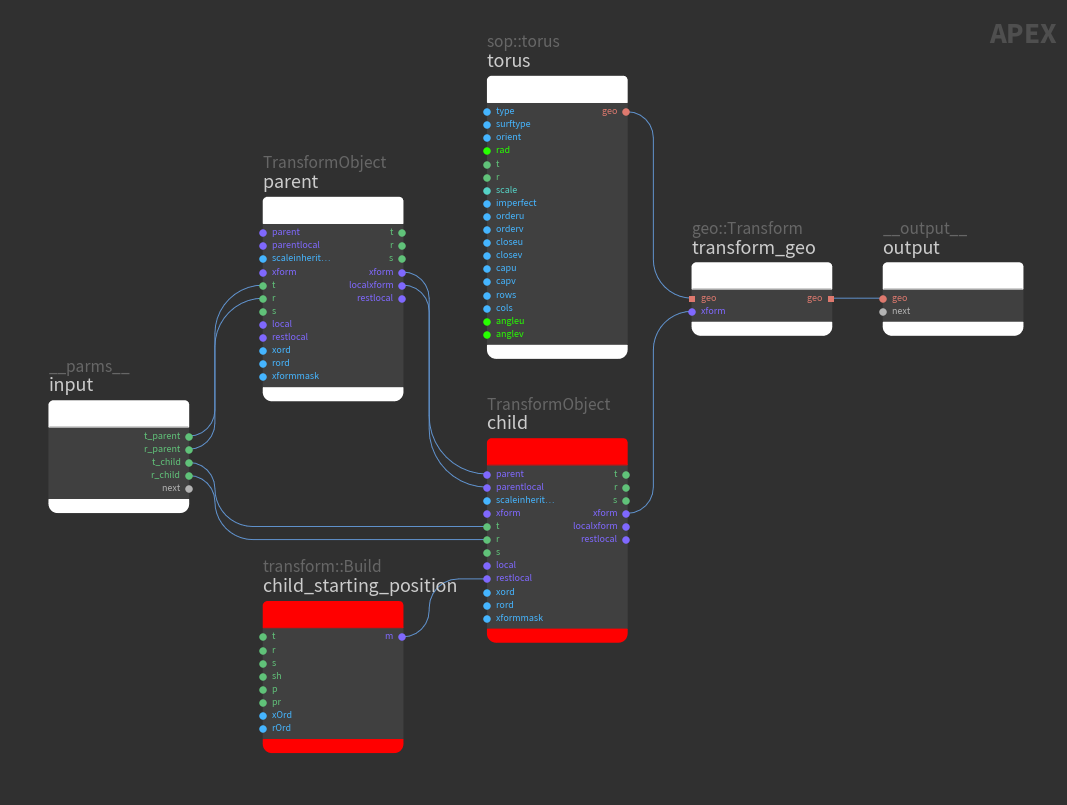
Create a parent-child control hierarchy Node
Description
childAdd a second TransformObject node to the graph and promote the t and r parameters. There are now two controls - the parent control and the child control.
A TransformObject node with something connected to its parent and parentlocal inputs is the child in a parent-child hierarchy. To create a parent-child hierarchy, make the following connections:
-
Parent TransformObject xform output → Child TransformObject parent input
-
Parent TransformObject localxform output → Child TransformObject parentlocal input
child_starting_positionCreates an offset for the
childTransformObject node so that the parent and child controls don’t sit directly on top of each other. To change the transform of the child control:-
Select the transform::Build node and press P to open the node parameter window.
-
Set the x-component of the transform parameter, t, to something like
1.0.
Connect
child_starting_positionto the restlocal input of thechildTransformObject node. restlocal defines the starting position of the child control in reference to the parent control - it is an offset to the parent control. -
Evaluate the rig logic using the animate state 
To see the parent-child hierarchy of controls, enter the animate state:
-
Connect the node network as in the controls example above.
-
Select the APEX Scene Animate SOP, and click
Animate on the left toolbar or press Enter in the viewport.
In the video below, we are in the animate state. The white dot on the left is the parent control. The white dot on the right is the child control.
The center of the torus sits at the child control because the position of the torus is driven by the child control.
Constraints 
In this example, we show how to break the parent-child behavior by creating a constraint.
Create the rig logic 
-
Start with the parent-child rig from the previous example.
-
Add a second child control (red nodes are new):
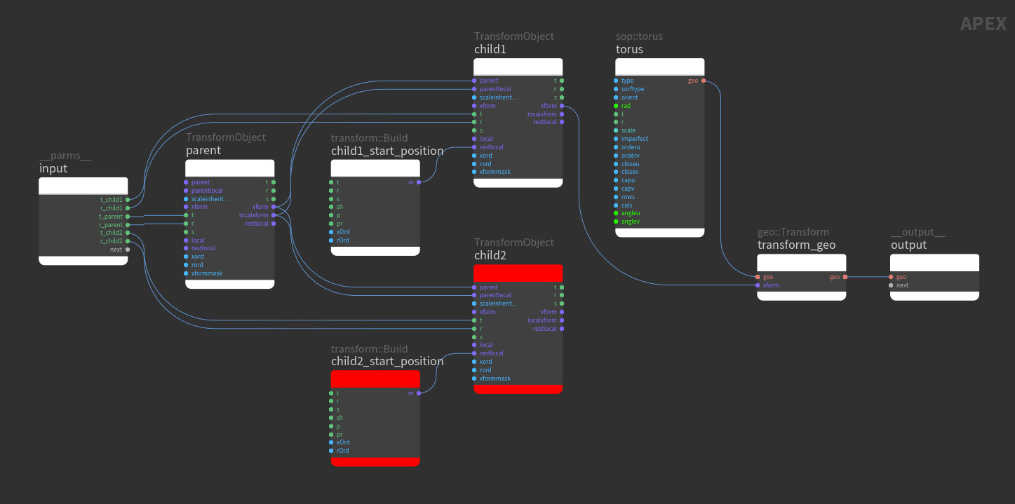
Create a second child control Node
Description
child2Promote the t and r parameters to create a second child control.
child2_start_positionCreates an offset for the new child control.
-
Select
child2_start_positionand press P to open the node parameter window. -
Set the x-component of the transform parameter, t, to a different value from the first child control (created in the previous example).
In the video below showing the animate state, the left control is the parent, the middle control is the first child, and the right control is the second child. Both child controls follow the parent.
Both child controls follow the parent -
-
Now constrain the
child2TransformObject control to a driver by connecting a transform::Build node (blue node nameddriver) to the xform input ofchild2. The TransformObject xform input is the world space transform and it overrides all the other inputs. If you connect something to xform, it will act like a constraint.-
Select the
drivernode and press P to open the node parameter window. -
Set the x-component of the transform parameter, t.
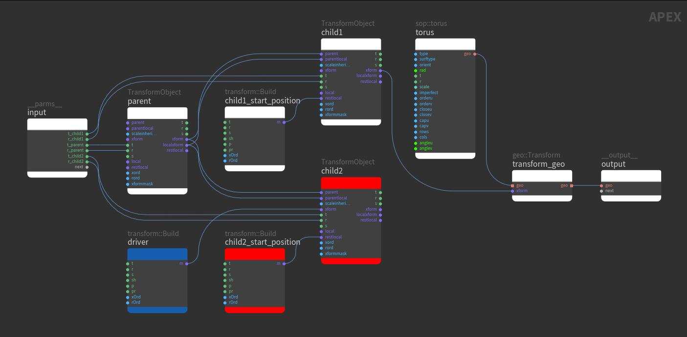
Constrain the second child control Note
If a TransformObject node is wired up as a child in a hierarchy, and you connect something to xform, the TransformObject will no longer follow its parent, but be constrained to the position of the xform input.
-
Evaluate the rig logic using the animate state 
In the video below, the child control in the middle follows the parent (left control) because it is not constrained. The child control on the right is in a parent-child hierarchy, but does not follow the parent because it has a constraining input (xform) that constrains its position to the xform position.
Note
If a TransformObject node is a child in a hierarchy and is also constrained (something is connected to its xform input), its localxform output will have a completely different value than if the TransformObject node is not parented. The local space is now “counter-animating” the movement of the parent to keep the control at its constrained position.
To constrain only one of translate, rotate, or scale while keeping the other transform components constant, see constrain one transform component.
Geometry deformation 
Pre-APEX, deforming geometry required a set of evaluation steps that were decomposed, in that the skeleton deformation had to be evaluated before the bone deformation. In the example below, we have a tube geometry that is being deformed. The ![]() Rig Pose SOP deforms the skeleton and the result of the skeleton deform evaluation goes into the bone deformation in the
Rig Pose SOP deforms the skeleton and the result of the skeleton deform evaluation goes into the bone deformation in the ![]() Bone Deform SOP.
Bone Deform SOP.
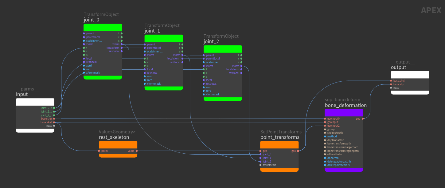
With APEX, we have the same steps to assemble and prepare the input elements to deform (blue nodes below), but the logic in the Rig Pose and Bone Deform SOPs from the pre-APEX setup are now in one place - the APEX graph in the bone_deform_rig node. The bone_deform_rig node builds up the rig logic, and the create_character node assembles the character elements in preparation for animation (see assemble character data for more information):
Create the rig logic 
The following is the rig logic in the ![]() APEX Edit Graph SOP,
APEX Edit Graph SOP, bone_deform_rig:
KineFX (Pre-APEX) |
APEX Graph Functionality |
Notes |
|---|---|---|
Rig Pose SOP |
FK hierarchy (green nodes), Animate skeleton via transforms (orange nodes) |
The three TransformObject nodes establish a 3-joint FK hierarchy, with Update the rest transforms of the TransformObject nodes to match the positions of the skeleton joints:
The world transforms of the Note In this example, the joint names on the skeleton were renamed from
The output of the SetPointTransforms node is the animated skeleton, which goes into the sop::bonedeform node. |
Bone Deform SOP |
Bone deformation (purple node) |
The three inputs of the Bone Deform SOP in the KinefX workflow correspond to the first three inputs of the sop::bonedeform APEX graph node. |
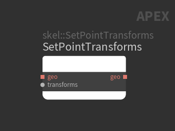
The table below gives more information on the SetPointTransforms and Value graph nodes.
Node |
Description |
|---|---|
|
SetPointTransforms is a skeleton deformer. It takes in transforms and applies them to skeleton joints. It is a special node in that the naming of the subports from the variadic input transforms is important. The subport names map to the joint names on the input skeleton (geo input on the SetPointTransforms node). For example, if one of the subports is named joint_0, changes made to the transforms going into the joint_0 subport will update Rename the subports on SetPointTransforms to match the skeleton joint names (joint names from the |
|
Value nodes |
The Value<Geometry> node makes a copy of the rest skeleton, and this copy is piped into SetPointTransforms. We need to make a copy of the rest skeleton because SetPointTransforms performs an in-place change of the geometry that is piped in. If a rest skeleton is piped into SetPointTransforms, SetPointTransforms will make changes to the rest skeleton. As a result, the rest skeleton will not be a rest skeleton anymore; it will be an animated skeleton. The rest skeleton is used as a reference for performing geometry deformation. The difference between the transforms of the rest and animated skeleton are calculated, and this difference is used to detemine how the geometry is deformed. If you don’t make a copy of the rest skeleton before it is piped into SetPointTransforms, SetPointTransforms will update the rest skeleton. The rest and animated skeletons will be the same, and no difference transforms will be applied to the geometry deformation. The example below shows what happens when the rest skeleton is piped directly into SetPointTransforms without first making a copy using a Value node. 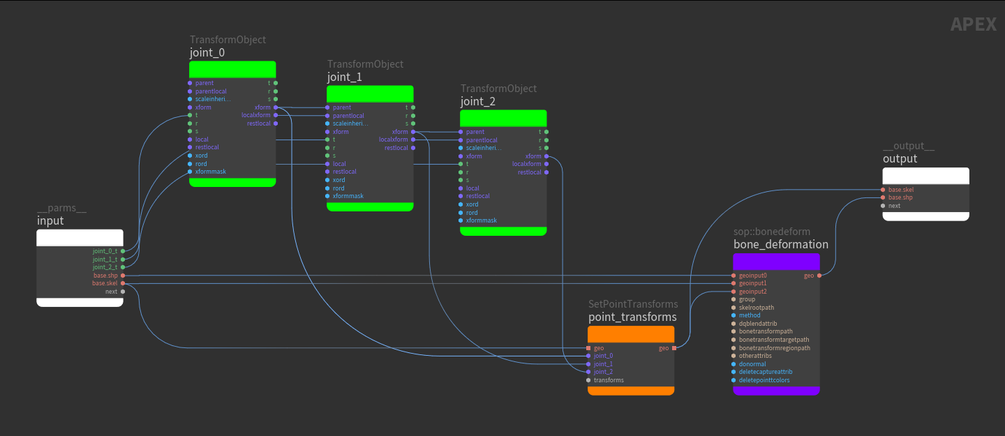
For the bone deformation to work as expected, we must use the Value<Geometry> node to make a copy of the rest skeleton. SetPointTransforms makes updates to the copy, and the animated skeleton is piped out of SetPointTransforms and into the 3rd input (animated skeleton), geoinput2, of the sop::bonedeform node. The original rest skeleton is piped into the 2nd input (rest skeleton), geoinput1, of the sop::bonedeform node. |
Evaluate the rig logic using the animate state 
The Pack Folder SOP is used to pack the character elements (tube geometry, skeleton, and rig) into a “character” that can be animated in the animate state. See assemble character data for information on how to name the character elements within the Pack Folder SOP.
To deform the geometry, enter the animate state:
-
Select the
APEX Scene Animate SOP in the network editor and turn on its display flag. -
Click
Animate on the left toolbar or press Enter in the viewport.
Note
If the geometry in the animate state looks mangled, it could be that the rest transforms in the rig graph are not set properly. To set the rest transforms based on the skeleton:
-
Make sure that the names of the TransformObject nodes match the names of the skeleton joints.
-
Select the APEX Edit Graph SOP in the network editor.
-
Click Update Rest Transforms From Skeleton in the parameter editor.
-
When the dialog comes up, select the Skeleton SOP in the network editor, which automatically selects the Skeleton node in the dialog.
-
Click Accept.
-
Select the APEX Scene Animate SOP and click Reset All.
-
Enter the animate state.
Constrain one transform component 
To constrain one particular transform component (translate, rotate, or scale) to a driver and keep the other components unchanged, use the xformmask port on the TransformObject node.
Set up a bit mask for the translate, rotate, and scale values. If you want to constrain the rotation of a joint to a driver’s rotation, set the Value<Bool> node for the rotation to True, and the Value<Bool> nodes for the translate and scale to False.
In the example below, the pink nodes set up the functionality of constraining one transform component to a driver.
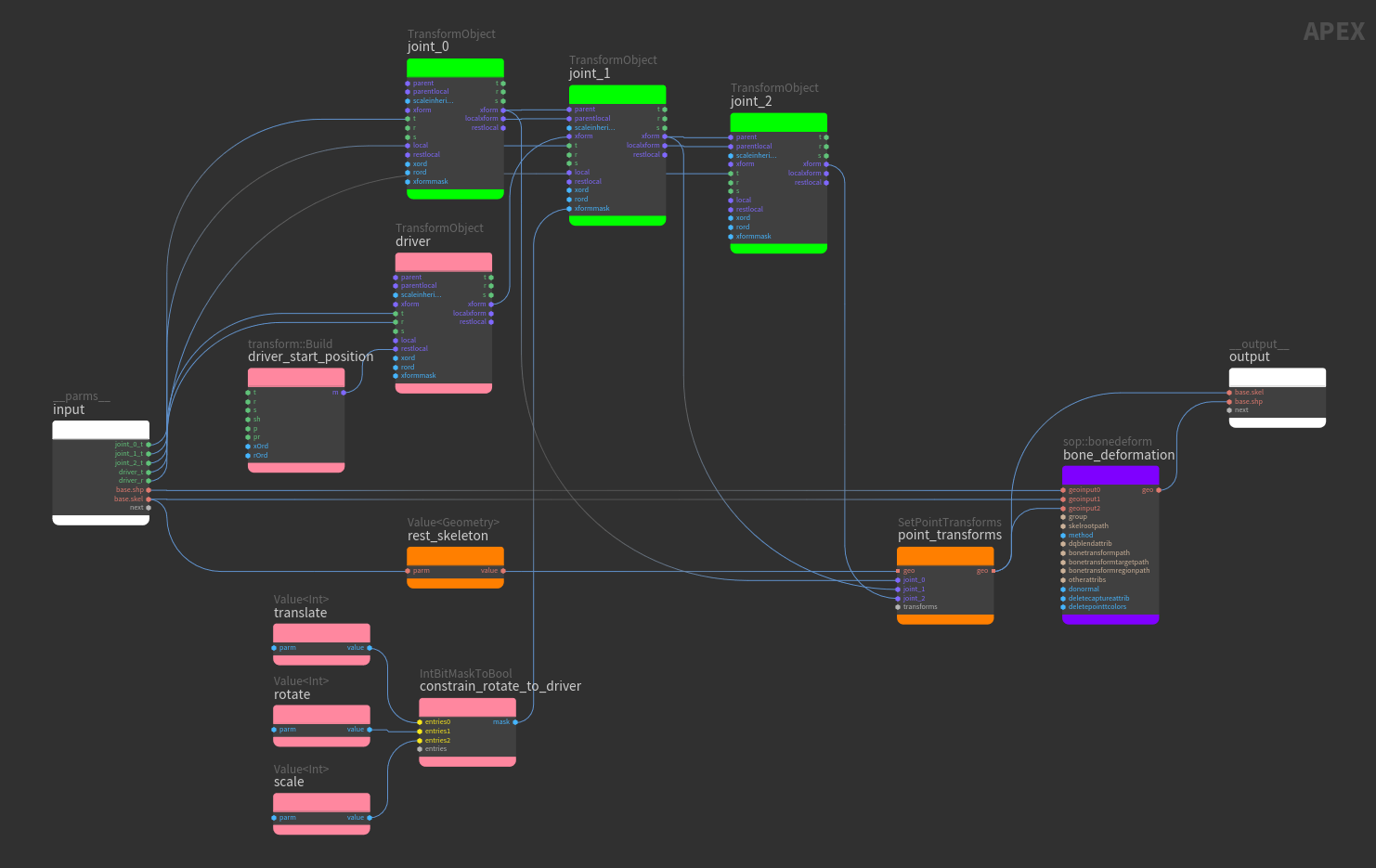
The translate and rotate values on the driver TransformObject node are promoted as controls and have the following functionality:
-
When the translate control of the
driveris changed,joint_1on the skeleton does not move because thejoint_1translate is not constrained to the driver. The tube geometry does not deform. -
When the rotate control of the driver is changed, the rotation of
joint_1updates along with the driver because thejoint_1rotate is constrained to the driver’s rotation. The tube geometry deforms with thejoint_1rotation.
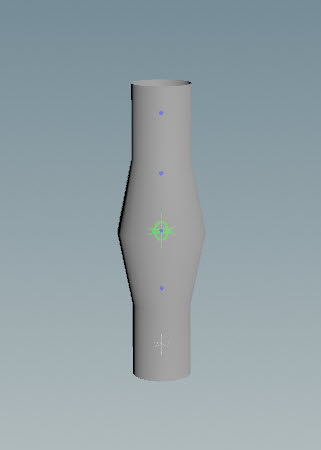
In the video below, when the driver translate is changed, the tube geometry does not deform. When the driver rotate is changed, the tube deforms with the rotation.
Abstract controls 
An abstract control is a control that can drive a float value or be used as a pivot point in the rig for posing purposes. An abstract control is not associated with a transform, unlike the controls created from TransformObject nodes. In the viewport, the interaction behavior of an abstract control is different from a regular control. For an abstract control, users drag the control to drive a float value. For a regular control, a transform handle is available to position and manipulate the control.
The AbstractControl graph node does not affect the functionality of the rig logic, nor does it get executed. It sits at the position specified by its xform input, and depending on its other input port connections, either drives a value or is used as a pivot point.
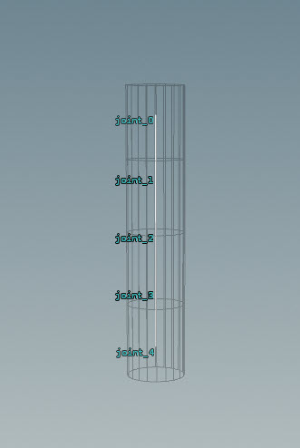
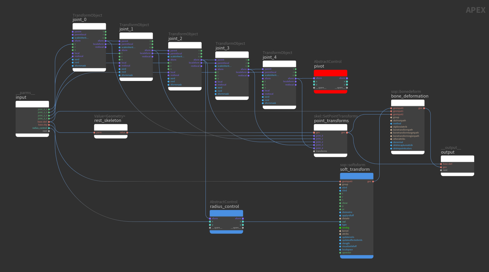
In this example, we start with a 5-joint tube geometry and build a network similar to the previous bone deformation example.
Two abstract controls are added to the bone deformation rig logic:
-
A pivot that sits at
joint_4(red node). -
A control that sits at
joint_2and drives the scale of the tube geometry aroundjoint_2(blue nodes).
Node |
Description |
||||||
|---|---|---|---|---|---|---|---|
|
The |
||||||
|
If something is connected to the xform input of an AbstractControl node, and its x and y input ports are unconnected, the AbstractControl node is interpreted by the viewport as a control that can be used as a pivot. The input to the xform port could come from any node as long as the input is a matrix. This is so that the AbstractControl node knows where to place the control. In this example, the xform output of The following behavior can be seen in the animate state:
|
||||||
|
The
|
||||||
|
If the x or y input/output port of an AbstractControl node is connected in the “path” of a promoted value, dragging on the abstract control in the horizontal or vertical direction drives the promoted value. The radius parameter, rad, on the The following behavior can be seen in the animate state: |
The following hotkeys change the drag behavior of the abstract control in the viewport.
Drag behavior |
Action |
|---|---|
Change control values by integer step size |
Hold ⌃ Ctrl while dragging. |
Change control values at a slower rate |
Hold ⇧ Shift while dragging. |
Change control values at a faster rate |
Hold ⌃ Ctrl + ⇧ Shift while dragging. |
Configure abstract controls 
Abstract control appearance 
To configure the size, shape, color, and position of abstract controls, use the ![]() APEX Configure Controls SOP.
APEX Configure Controls SOP.
-
In the APEX Configure Controls SOP, click
beside Control Configs to add a set of configurations for each abstract control. Setting
Parameter
Rig name
Specify the rig to configure the abstract controls for in the Rig Source parameter. The name of the rig is set in the
Pack Folder SOP. See assemble character data for information on how to name character elements within the Pack Folder SOP.Controls to configure
In the Control Group parameter, specify the name of the abstract control, or use the APEX path pattern syntax to specify groups of controls.
Control shape, size, and color
Turn on the desired Use Shape Override, Use Shapeoffset, and Use Color parameters.
-
To view the configured abstract controls, enter the animate state:
-
Select the
APEX Scene Animate SOP in the network editor and turn on its display flag. -
Click
Animate on the left toolbar or press Enter in the viewport.
-
Abstract control properties 
Abstract control properties define how the control behaves in the viewport. These properties are stored in the properties dictionary attribute of the AbstractControl node. The properties dictionary contains a set of nested dictionaries with the following hierarchy:
control:
    parms:
        <property1>,
        <property2>,
        ...
control
A dictionary that contains information on how to configure the control, for example, how the control should look in the viewport and the default parameters of the control. Information on control shapes is also stored in this dictionary.
parms
Inside the control dictionary is another dictionary called parms, which stores the default parameters that determine the behavior of the control.
The table below lists the properties that can be configured for an abstract control:
Property |
Type |
Description |
|---|---|---|
x_min, x_max |
|
Defines the default minimum/maximum value for the control when dragging in the horizontal direction. If not defined, the default minimum and maximum values are -10 and 10. |
y_min, y_max |
|
Defines the default minimum/maximum value for the control when dragging in the vertical direction. If not defined, the default minimum and maximum values are -10 and 10. |
lock_range |
|
When set to |
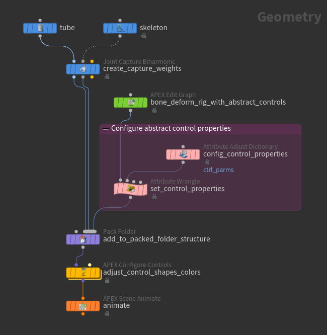
Abstract control properties can be configured using the ![]() Attribute Adjust Dictionary SOP and
Attribute Adjust Dictionary SOP and ![]() Attribute Wrangle SOP. The Attribute Adjust Dictionary SOP is used to create a dictionary of control properties. This dictionary is then set on the
Attribute Wrangle SOP. The Attribute Adjust Dictionary SOP is used to create a dictionary of control properties. This dictionary is then set on the properties attribute of the AbstractControl node using the Attribute Wrangle SOP.
Node |
Description |
||||||
|---|---|---|---|---|---|---|---|
Attribute Adjust Dictionary SOP |
Creates a dictionary of abstract control properties.
|
||||||
Attribute Wrangle SOP |
Sets the dictionary of properties on the abstract control’s Set the Group parameter to In the VEXpression textbox, enter the following VEX code: dict parms = detail(1, '<Attribute Name parameter>'); dict ctrl; ctrl['parms'] = parms; d@properties['control'] = ctrl; The Note The dictionary created by the Attribute Adjust Dictionary SOP can be set to any name (in the Attribute Name parameter). However, the dictionaries within the abstract control’s The following hierarchy of data is created on the abstract control’s control:
parms:
x_min,
x_max,
...
The abstract control’s
|
Attributes, callbacks, and properties 
APEX graph geometry have the following attributes.
Name |
Class |
Type |
Description |
|---|---|---|---|
|
point |
|
Name of the node. |
|
point |
|
Callback name of the node. |
|
point |
|
Color of the node. |
|
vertex |
|
Name of the port. |
|
vertex |
|
Subport name or renamed ports. |
|
vertex |
|
Index number of the port. |
|
point |
|
Dictionary of default values for ports. |
|
point |
|
Array of strings that are matched using the APEX path pattern syntax via |
|
point |
|
Dictionary of additional metadata for the node. |
There are special callback names for some of the graph elements.
Node |
Callback name |
|---|---|
Graph input node |
|
Graph output node |
|
Subnet |
|
Sticky note |
|
Properties 
Properties on graph nodes store custom information that could be used at a later point in the graph. They are stored in a dictionary attribute called properties. Users can add and modify data in the properties dictionary using graph::UpdateNode and graph::UpdateNodeProperties.
Note
Properties are only used for nodes; there are no port properties.
The properties dictionary also contains predefined entries that store information on control shapes, rig parameter limits, and rig/skeleton mapping. Users can use and modify this information. The predefined entries are shown below:
{
    control: {
        color: Vector3
        shapeoffset: Matrix4
        shapeoverride: String
        visibility: Int
    }
    max:<parameter_name>: Vector3
    min:<parameter_name>: Vector3
    max_lock:<parameter_name>: Vector3
    min_lock:<parameter_name>: Vector3
    mapping:<skeleton or rig>: String
}
The mapping property can be set using the ![]() APEX Map Character SOP, and the other properties can be set using the
APEX Map Character SOP, and the other properties can be set using the ![]() APEX Configure Controls SOP.
APEX Configure Controls SOP.
Property |
Type |
Description |
|---|---|---|
control |
|
A dictionary that contains information on how the control looks in the viewport. |
color |
|
The color of the control. |
shapeoffset |
|
The position of the control. |
shapeoverride |
|
The shape of the control. |
visibility |
|
Whether the control is visible in the animate state. |
max, min |
|
A soft limit on the rig transform parameters. The Vector3 values are the limits on the x, y, and z values of the parameter. The user can control whether or not to enforce the limits or use the limits as a visual indicator in the animate state. See transform limits for more information. The format of the max and min properties is:
|
max_lock, min_lock |
|
A hard limit on the rig transform parameters. The Vector3 values are the limits on the x, y, and z values of the parameter. This cannot be turned off in the animate state. See transform limits for more information. The format of the max_lock and min_lock properties is:
|
mapping |
|
Specifies the mapping between rigs or skeletons to TransformObject nodes. This is useful for mapping skeleton joints to controls, or in the case where one rig drives another, mapping the controls between two rigs. This mapping information is stored on the TransformObject node. The format of the mapping property is:
|
An example of the predefined entries in the properties dictionary:
{
    "control":{
        "color":[0.5,0,1],
        "shapeoffset":[0.3,0,0,0,0,0.3,0,0,0,0,0.3,0,0,0,0,1],
        "shapeoverride":"torus",
        "visibility":1
    },
    "max:t":[5, 5, 5],
    "min:t":[-5, -5, -5],
    "max_lock:t":[10, 10, 10]
    "min_lock:t":[-10, -10, -10],
    "mapping:Base.skel":"lowerarm_l"
}
How-to 
| To... | Do this |
|---|---|
|
Fetch numerical values from a graph |
The output dictionary can be viewed on the geometry spreadsheet by selecting See the example for adding two values. |
|
Display geometry from a graph |
See the example for modifying geometry. |
|
Add a control |
For the parameters you want to turn into controls, promote the input parameters on the TransformObject node by connecting the parameters to the graph See the example for adding controls. |
|
Create a parent-child hierarchy |
Make the following connections between two TransformObject nodes:
See the example for creating a parent-child hierarchy. |
|
Set the starting position of the child control in reference to the parent control |
Connect a transform::Build node to the restlocal input of the child TransformObject node. restlocal defines the starting position of the child control in reference to the parent control - it is an offset to the parent control. |
|
Create a constraint |
To constrain a TransformObject node to a driver, connect the driver to the xform input of the TransformObject node. See the example for creating a constraint. |
|
Constrain one transform component |
Use a BoolToIntBitMask node, and Value nodes for the translate, rotate, and scale components to create a bit mask that determines the particular transform component to constrain. Connect the BoolToIntBitMask node to the xformmask input of the TransformObject node you want to constrain. See the example for constraining one transform component. |
|
Create a rig hierarchy that corresponds to a skeleton |
Use the Import KineFX Skeleton button on the |
|
Update the rest positions of the rig hierarchy from a skeleton |
Use the Update Rest Transforms From Skeleton button on the APEX Edit Graph SOP. |
|
Delete a wire on the graph |
Hold Y and or Select the wire and press Delete. |
|
Change the parameter values on a graph node |
Select a graph node and press P to bring up the APEX node parameter window. |
|
Rename a subport on the graph |
|
|
Keep a graph visible in the APEX network view |
Unpin the graph if you want the APEX network view to display the graph of whichever node is selected in the network editor. |
Notes about naming 
-
On the SetPointTransforms node, subports from the variadic input transforms must match the joint names on the input skeleton (geo input on the SetPointTransforms node).
-
The names of TransformObject nodes do not need to match the skeleton joint names. However, if you want to use the Update Rest Transforms From Skeleton button on the
APEX Edit Graph SOP, the TransformObjects nodes need to match the skeleton joint names.