| On this page | |
| Since | 21.0 |
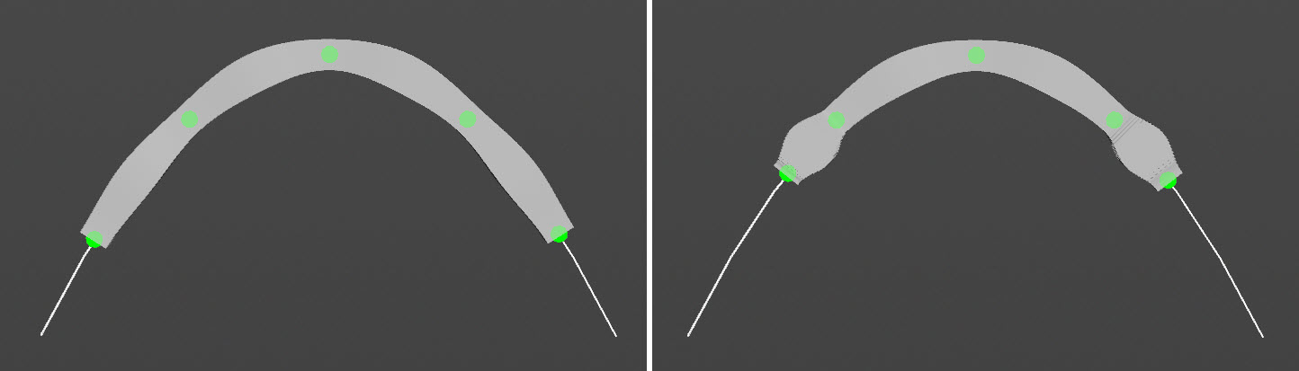
Generates a spline from a number of input control matrices. The position of the control matrices defines the shape of the generated spline, while the upper 3×3 transform of the matrices defines the framing of the spline in the proximity of the CV. The spline is then sampled into numsamples interpolated transform samples.
This node combines the functionality of ![]() rig::ControlSplineFromArray and
rig::ControlSplineFromArray and ![]() rig::SampleSplineTransformsToArray. The sections below describe the spline functionality that is available in this node.
rig::SampleSplineTransformsToArray. The sections below describe the spline functionality that is available in this node.
Control spline 
The control spline is the spline that is sampled, and it is created using the values from the cvs, order, and splinetype ports.
The control matrices (cvs) contain the position of the spline’s CVs, as well as the
orientation of the spline. The orientation of each CV is applied at the
normalized curve parameter curveu = vtxnum/numvtx (which is generally in
the proximity of the CV).
The order of the spline (order) affects the flexibility and shape of the curve. Order 3 and 4 curves are popular choices for ensuring that each CV has a relatively local impact on the shape of the curve while simultaneously producing smooth shapes. An order 2 curve is equivalent to a linear polyline.
Splines can be created as either a Bezier or NURBS curve according to the value of splinetype. Each spline type has its own advantages. Bezier curves pass through the first CV, last CV, and every knot (the CVs representing the junction points of curve segments in a compound curve). However, Bezier curves can be restrictive in that they require a specific number of CVs to form a valid curve. NURBS curves are more flexible in the number of CVs required to form a valid curve (they just need a minimum of order CVs). However, NURBS curves only pass through the first and last CVs, approximating the position of the rest of the CVs.
Bezier Curve Construction
Each segment of a Bezier curve requires that <number_of_cvs> = order.
Compound curves share a CV between their curve segments, so each additional
curve segment requires an additional order-1 CVs. This requirement can
be expressed by the equation <number_of_cvs> % (order-1) == 1.
For example, if an order 4 Bezier curve is created with two curve segments, it would require 4 CVs for the first curve segment and 3 CVs for the second curve segment (since the second curve segment shares its first CV with the first curve segment). This amounts to a total of 7 CVs.
Spline samples 
The samples are output on the xforms port, and the number of output samples is determined by the numsamples value. The orientation of a sample is interpolated from the coordinate frames of the control spline surrounding the sample.
By default, samples are built such that they can be used as a joint chain. In particular, their interpolated orientation is realigned so that the sample’s local look at axis, lookataxis, aligns with the next sample’s position. The lookataxis of the last sample coincides with the tangent of the curve. The choice of look at axis alignment can be adjusted with the lookattype port.
lookattype |
Look At Type |
|---|---|
0 |
Next Sample The look at axis aligns with the next sample in the output joint chain. |
1 |
Curve Tangent The look at axis aligns with the curve’s tangent vector. |
In addition to the xforms array, the samples are also available via the
outgeo output port as a geometry. The outgeo geometry has transform point attributes that contain the orientation (and scaling) of the joints.
Spline offsets 
A spline offset is the offset from the beginning of the spline to a specific point along the spline. Offsets are defined by a value (specified in ports startoffset, endoffset, twists, and pins) and its unit (startinterp, endinterp, twistinterps, pinintersp). The unit of the offset is referred to as its “interpretation”.
interp |
Interpretation |
|---|---|
0 |
Unit Parametric The offset value is interpreted as a normalized parametric value with 0 representing the beginning of the spline and 1 representing the end of the spline. Unit parametric offsets are useful for sampling in the parametric domain while remaining more invariant to changes to the spline’s parameterization (for example, adding or removing a CV from the control spline). |
1 |
Unit Arclength The offset value is interpreted as a normalized arclength. The offset represents the percentage of the arclength along the spline. A value of 0 represents the beginning of the curve and a value of 1 represents the end of the curve. Unit arclength offsets are convenient for maintaining a relative distance when the spline changes length. |
2 |
Parametric The offset value is interpreted as a parametric value. Parametric values precisely identify a position along a spline and may remain more localized to changes to the spline’s length or shape. |
3 |
Arclength The offset value is interpreted as an arclength. Arclength offsets are useful for specifying an offset at a specific distance along the spline even when the length of the spline changes. |
When unspecified, the interpretation is assumed to be “Unit Parametric”.
The startoffset and endoffset values (along with their corresponding startinterp and endinterp values) restrict the active domain of the spline used for sampling. Various effects can be accomplished by modifying these parameters, including:
-
Stretching a joint chain along a spline:
-
Transporting a fixed length joint chain along a spline:
Fixed length splines 
A fixed length spline is a spline with user-defined lengths between its output samples. Fixed length splines are created when the restlengths port is provided with inputs, and the stretch port has a value of 0. If we consider the output samples to represent a joint chain, each restlengths value is the distance between the corresponding joint and the next joint in the joint chain.
Rest lengths can be set on a joint-by-joint basis in order to support non-uniform lengths:
If the number of restlengths entries does not match the number of output samples, the last user-provided rest length is repeated as many times as necessary to provide all the joints with a rest length value. To produce a joint chain where all the joints have a uniform rest length, only a single value needs to be input to restlengths.
A fixed length joint chain can be offset along a spline using a pin. If the joint chain reaches the spline’s startoffset or endoffset, the joints will begin to collapse on each other. However, if overshoot is set to True, the joint chain will not collapse when reaching the spline offsets, and could even overshoot the spline completely.
Stretchy splines 
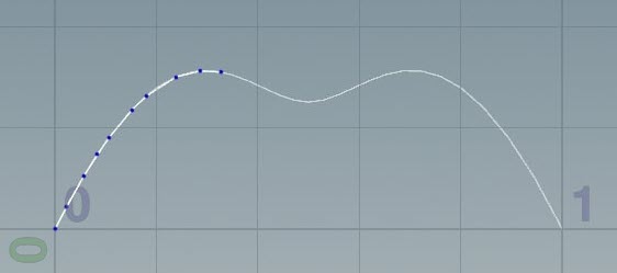
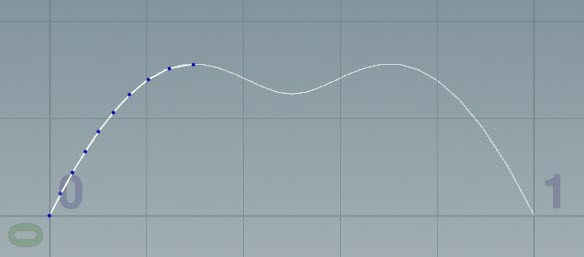
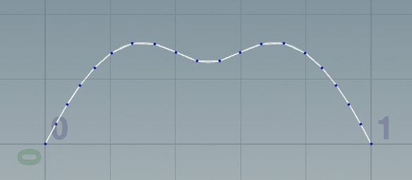
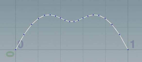
A stretchy spline is a spline that stretches its output samples along its available length, evenly distributing the samples between the startoffset and endoffset of the spline according to the stretchtype.
stretchtype |
Stretch Type |
|---|---|
0 |
Arclength Samples are distributed at even arclength intervals.
|
1 |
Parametric Samples are distributed at even parametric intervals.
|
Stretchy behavior occurs in a few scenarios:
-
The restlengths port is unconnected.
-
The stretch port has a value of 1.
-
Spline pins stretch the output joints.
When a fixed length spline solution exists, the stretch port controls the blending of the fixed length and stretchy solutions. A value of 0 corresponds to no stretching and a value of 1 is completely stretched. Intermediate values provide a blend.
Stretch and squash 
You can apply stretch and squash scaling factors to the output transforms by adjusting the stretchscale and squashscale values respectively. If the value is greater than 1, stretching occurs when the samples are stretched beyond their rest lengths, while squashing occurs when the samples are closer together than their rest lengths. A value of 1 indicates that no additional stretch or squash scaling is applied.
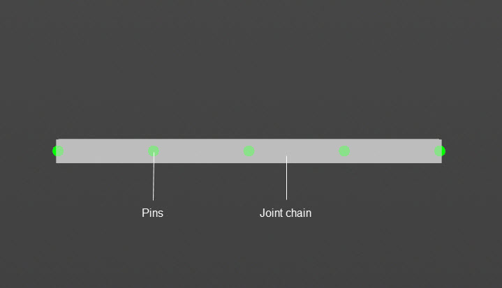
In the stretchsquashtype port, you can specify the type of stretch and squash scaling to apply to the joint segments. To illustrate the different types of stretch and squash in the table below, we start with a joint chain at its rest length containing evenly spaced pins, then we stretch the joint chain:
stretchsquashtype |
Stretch Squash Type |
|---|---|
0 |
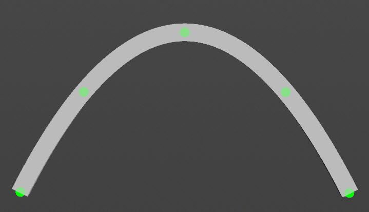
Joint Length The amount stretch or squash experienced by an individual joint is localized to its neighboring joints in the joint chain. If the distance between its neighbors increases, it will stretch. If the distance decreases, it will squash. Stretch and squash is computed using the ratio of the joint’s length to its rest length (for example, when the joint’s length is greater than its rest length, stretching occurs):
As you move the interior pins around, stretching and squashing occurs along the joint chain. Since each joint is treated independently, this tends to result in hard transitions between the stretched and squashed segments: 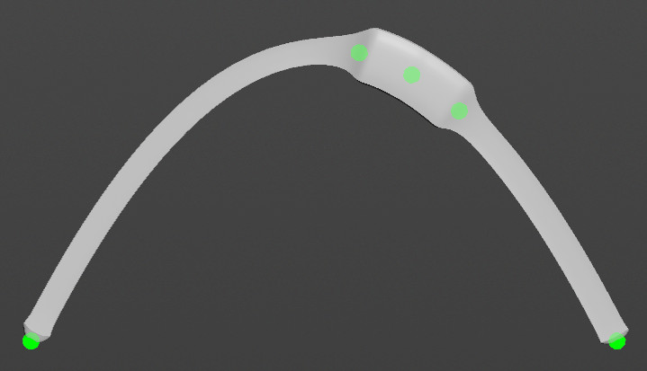
|
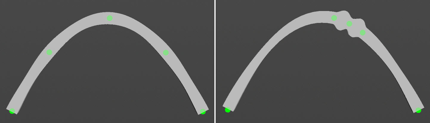
1 |
Smoothed Segments Stretch and squash is computed in the same way as “Joint Length” mode, but is only applied between the pins, so the scaling at the pins is unaffected by stretching and squashing: 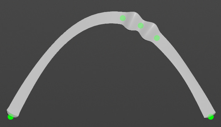
This mode may be best suited for fixed length joint chains that slide along the spline. In this case, stretching and squashing within the fixed length joint chain will look natural, and stretching or squashing at the ends of the joint chain will have a local effect. Note If you intend to have the joint chain stretched most of the time, this mode may not be the best option because the joint chain will bulge out at the pin locations since the scale at the pins is unaffected by the stretching. The bulging is noticeable if the joint chain is evenly stretched (the pins are evenly spaced, so each joint chain segment is stretched the same amount). Changing the number of pins would affect the number of bulges in the joint chain. 
|
2 |
Joint Chain Length The amount of stretch or squash experienced by an individual joint is affected by the length of the joint chain in addition to the joint’s distance from its neighboring joints. Stretch and squash is computed using the ratio:
As you move the interior pins around, stretching and squashing occurs between the pins, and the scale at the pins is unaffected by the stretch and squash scaling. This is similar to “Smoothed Segments” mode. As you stretch or squash the entire joint chain by changing its length, on the other hand, the entire joint chain is scaled, including the pins. As a result, when the joint chain is evenly stretched, this mode avoids the bulges seen in “Smoothed Segments” mode. The images below show a comparison between Joint Length mode, Smoothed Segments mode, and Joint Chain Length mode: 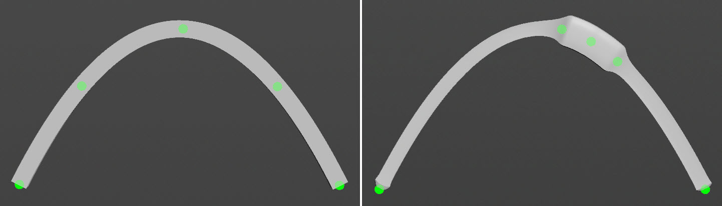
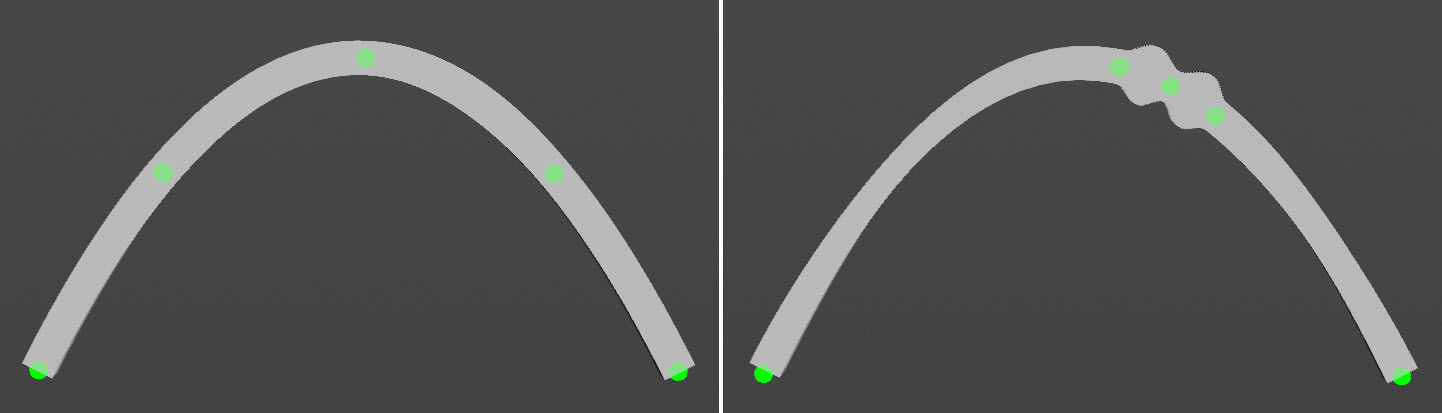
Because changes to the length of the joint chain affects the scaling at the pins, this mode may be best suited for fixed length joint chains or joint chains that remain fully stretched. |
3 |
Spline Length The amount of stretch or squash experienced by an individual joint is affected by the length of the spline curve in addition to the joint’s distance from its neighboring joints. Stretch and squash is computed using the ratio:
Note The spline’s rest length is assumed to be the joint chain’s rest length. In the image below, the joint chain is at its rest length, and the spline length has increased. This introduces squashing. To arrive at this result, imagine that the joint chain is stretched along the full length of the longer spline while keeping its original scaling, then each segment is squashed into the positions shown below: 
This mode is useful for stretchy joint chains, especially when you want to have localized stretching and squashing at the end segments of the joint chain (in addition to the scaling at the interior segments). If you adjust the end segments in this mode (changing the length of the joint chain), the joints along the entire joint chain are not scaled as in the case of “Joint Chain Length” mode: 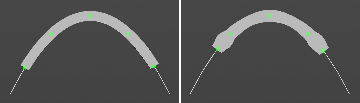
This mode may not be well suited for fixed length joint chains because the length of the spline curve affects the scaling at the pins. |
Pins 
A pin constrains a fixed length joint chain’s position to an offset on the spline. If there are no pin inputs, an implicit pin is created to constrain the start of the joint chain to the start of the spline curve.
In the following example, we cycle between pinning the start, middle, and end of the joint chain to the middle of the spline:
You can add an arbitrary number of pins. In the following example, there are 3 pins. The first pin constrains the start of the joint chain to the unit arclength 0.25. The second pin constrains the end of the joint chain to unit arclength 0.75. The third animates the middle of the joint chain between 0.35 and 0.65 unit arclengths on the spline:
You can also use pins to grow a fixed length spline from a starting point. In the following example, a single pin constrains the end of the joint chain to the end of the spline. The value of endoffset is initially set to 0, and as its value is increased, we can see the joint chain growing out from the starting position:
Note
Pins are clamped between startoffset and endoffset.
Twists 
The control spline gives the curve an initial orientation. If the rotation of a control frame extends beyond 180 degrees, however, the control matrix will not be able to account for the extended rotation. To help address this issue, additional rotations can be added directly to the output joint chain (as opposed to the control frames) via the twists port. As long as a single joint does not twist beyond 180 degrees, the rotation should remain stable.
In the following example, a single twist is created at the end of the spline. Its rotation is animated from 0 to 2*PI radians:
An arbitrary number of twist entries can be added to the node. In the following example, a twist of 0 radians is added at 0.25 arclength and 0.75 arclength, and an animated twist of 0 to 2*PI radians is added at 0.5 arclength:
Inputs 
                cvs:
                    VariadicArg<Matrix4>
A list of CVs, provided as Matrix4 transforms, that specify the position of the CVs, as well as a coordinate frame for the spline in the vicinity of the CV.
                splinetype:
                    Int
The type of spline curve to create from the input CVs. A value of 0 creates a Bezier curve and a value of 1 creates a NURBS curve. The default is a Bezier curve.
                order:
                    Int
The order of the generated spline curve. As the order of the spline increases, each CV has more global impact on the shape of the curve. Order 3 and 4 curves are popular choices to ensure that each CV has a relatively local impact on the shape of the curve while simultaneously producing smooth shapes. An order 2 curve is equivalent to a linear polyline.
                numsamples:
                    Int
The number of output samples to evaluate.
                lookataxis:
                    Vector3
A local space vector that aligns the sample toward the next sample in the output joint chain. The default value is the X axis, so by default, the X axis of the sample’s transform points toward the next sample.
For stable results, it is important that the orientation of the control spline’s transform attribute use the same axis as its look at axis.
                lookattype:
                    Int
Determines how the lookataxis of a sample is aligned. With the default value of 0, the lookataxis aligns toward the next sample in the joint chain. With a value of 1, the lookataxis aligns with the curve’s tangent vector.
                smooth:
                    Bool
If set to True, uses smooth-step smoothing when interpolating the output transform’s orientation. The default value is False.
                stretchtype:
                    Int
Determines if the samples are evenly stretched parametrically or by arclength. A value of 0 is Arclength, and a value of 1 is Parametric. The default is Arclength.
                stretch:
                    Float
Blends between a fixed length solution and a stretchy solution. A value of 0 represents a fixed length solution, a value of 1 represents a stretchy solution, and intermediate values are a blend of the two solutions. Defaults to 1 (stretchy solution).
                stretchsquashtype:
                    Int
The stretch and squash model to apply to the joint segments when the stretchscale or squashscale scaling factors are used. By default, the “Joint Length” stretch and squash type is used.
                stretchscale:
                    Float
A scaling factor to apply to the output transforms when the samples are stretched (further apart than their rest lengths). The default is 1, which indicates no additional scaling. Valid scaling factors are greater than 1.
                squashscale:
                    Float
A scaling factor to apply to the output transforms when the samples are squashed (closer together than their rest lengths). The default is 1, which indicates no additional scaling. Valid scaling factors are greater than 1.
                startoffset:
                    Float
Restricts the start of the spline’s active domain to a specific offset along the spline. The default is 0, which when paired with the default startinterp, means the spline’s active domain starts at the beginning of the spline curve.
                startinterp:
                    Int
The interpretation of the startoffset port. The default interpretation is Unit Parametric.
                endoffset:
                    Float
Restricts the end of the spline’s active domain to a specific offset along the spline. The default is 1, which when paired with the default endinterp, means the spline’s active domain ends at the end of the spline curve.
                endinterp:
                    Int
The interpretation of the endoffset port. The default interpretation is Unit Parametric.
                overshoot:
                    Bool
If set to True, and a fixed length joint chain extends beyond startoffset or endoffset, the joint chain maintains its length rather than collapse at the offset. The default is False.
                restlengths:
                    FloatArray
The distance between an output sample and the next sample in the joint chain. Each restlengths entry corresponds to the rest length of a single output sample.
If the number of restlengths entries does not match the number of output samples, the last user-provided rest length is repeated as many times as necessary to provide all the joints with a rest length value. To produce a joint chain where all the samples have the same rest length, it is only necessary to provide a single restlengths value, which is repeated for all the samples.
In the absence of user-provided rest lengths, the rest lengths are set according to their stretched solution.
                twists:
                    Vector2Array
Additional rotations applied about the sample’s local lookataxis. Twists are expressed as a Vector2. The first vector component is the rotation expressed in radians. The second vector component is the offset along the spline at which the twist is applied. By default, the offset’s interpretation is Unit Parametric, but this can be changed by setting the corresponding entry on the twistinterps port.
                twistinterps:
                    IntArray
Each twistinterps entry sets the offset interpretation of the corresponding entry on the twists port. If there are no inputs to twistinterps, the default offset interpretation is Unit Parametric.
If the number of twistinterps entries does not match the number of twists entries, the value of the last twistinterps is repeated as many times as necessary to give each twists entry a valid interpretation. This behavior can be used to conveniently set all the twists offset interpretations by adding a single entry to twistinterps with the desired interpretation.
                pins:
                    Vector2Array
Constrains a position on a fixed length joint chain to an offset on the spline. The position on the joint chain and offset on the spline are specified as a Vector2. The first vector component is the position on the output joint chain, and its interpretation is always Unit Arclength. The second vector component is the offset along the spline. By default, its interpretation is Unit Parametric, but this can be changed by setting the corresponding entry on the pininterps port.
                pininterps:
                    IntArray
Each pininterps entry sets the spline offset interpretation of the corresponding entry on the pins port. If there are no inputs to pininterps, the default spline offset interpretation is Unit Parametric.
If the number pininterps entries does not match the number of pins entries, the value of the last pininterps is repeated as many times as necessary to give each pins entry a valid interpretation. This behavior can be used to conveniently set all the pins spline offset interpretations by adding a single entry to pininterps with the desired interpretation.
Outputs 
                arclength:
                    Float
The arclength of the control spline spanned by the resampled spline. If overshoot is set to True, and the samples extend beyond the end of the spline, the additional distance is included in the arclength.
                xforms:
                    Matrix4Array
The sampled transforms. The number of samples is determined by the numsamples port.
| See also |