| On this page |
Overview 
You can create your own custom constraints by building a constraint graph and configuring the graph so the animate state knows how to pick it up.

The steps for creating a custom constraint are:
-
Create a constraint graph using an
 APEX Graph SOP or APEX Script.
 The inputs to the constraint graph are control transform matrices and other parameters that affect the constraint. In the example constraint graph below, the radians port on the graph input node is a parameter that the user can control in the animate state. The start and end ports are transform matrices whose data come from the driver or driven (constrained) controls. The constraint graph must also have an output node with an xform port, which is the new world space transform of the driven control.

Example constraint graph -
Configure the constraint graph using an
 APEX Configure Graph SOP, which specifies where the constraint’s input data comes from.
 -
To be able to add the constraint in the animate state:
-
Use a
 Pack Folder SOP to add the constraint graph to the
 /constraints/libraryfolder in the character folder structure. Graphs that are added to this folder are picked up by the animate state as a constraint.or
-
Save the graph as a .bgeo file and add it to the constraints registry in the Houdini path, for example,
$HOUDINI_PATH/apexconstraint/<constraint>.bgeo. Graphs in this registry are picked up by the animate state as a constraint.
-
Pin constraint 
In this example, we create a pin constraint that keeps a control at a certain position. We then test the constraint on the  Electra test geometry:

-
On the
Electra SOP, set Output to APEX Scene. -
Use an
APEX Graph SOP to create a graph that defines the functionality of the pin constraint. The pin constraint graph takes in a transform matrix and pipes out that same transform matrix: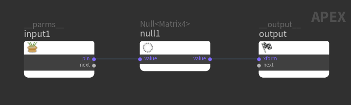
Pin constraint graph -
Rename the graph input port to pin and the graph output port to xform.
 click the port name to rename it.
 -
The pin input port brings in the transform of the driven control at the time the constraint is created.
-
The xform output port is the transform of the driven control after the constraint is created.
-
-
The
APEX Configure Graph SOP configures the constraint graph so that it can be brought into the animate state. On the APEX Configure Graph SOP:-
Set Mode to Constraints.
-
In the Name parameter, specify a name for the constraint. In our example, we set Name to “
Pin Test”.
-
-
Specify where the input data for the pin constraint comes from. On the APEX Configure Graph SOP:
-
In the Constraint Configuration section, click
 beside Input Bindings.
 -
The name of the input port is set in the To Port parameter. In our example, we set To Port to
pin. -
The control to link to the input port is a driven control, so set From Control to Driven Control.
-
We want the pin input port to be locked to the control’s position when the constraint is created, so set Driven Data to Static Transform.
-
-
Add the pin constraint to the animation scene - on the
Pack Folder SOP:-
Set Parent Folder to
/constraints/library. This adds the pin constraint to the/constraints/libraryfolder in the character folder structure. The animate state picks up custom constraints from this folder. -
Specify a name for the pin constraint graph. In our example, we set Name to
pin_test. The Type parameter must be set tograph. In the rig tree view, the following character folder structure is displayed:/ -- constraints/ -- library/ -- pin_test.graph -- electra.char/ ...
-
-
Enter the animate state - select the
 APEX Scene Animate SOP, turn on its display flag, and click
  Animate on the left toolbar.
 -
In the animate state parameters, Constraint tab, Parameters section, the Pin Test constraint appears as one of the options in the Constraint drop-down menu. Select the Pin Test constraint.
-
Select the control to pin and press H over the viewport. A pin constraint is created, which keeps the control at its position:
Pin the chest control Note
To see the effects of the pin constraint on Electra’s chest control, set the stretch value of Electra’s spine to 1 using the spine’s
 menu.
menu.
Configuration control for Electra’s spine
-
Constrain a control to a sine function 
In this example, we constrain the x-component of a ball’s position to a sine function.

-
The
 APEX Scene Add Prop SOP adds the ball geometry to an animation scene. In the Prop Name parameter, set the name of the ball that will appear in the selection sets.
 -
The graph in the
APEX Graph SOP defines the functionality of the sine constraint:
Sine constraint graph -
Rename the matrix graph input port to control and the graph output port to xform.
-
The control input port brings in the position of the ball control.
-
The
 transform::Explode node breaks out the translate component of the ball control’s transform, the
  Sine function is added to the x-value of the ball’s translation, and transform::Build builds back the ball’s transform with the updated translation.
 -
The radians input port is a parameter that controls the angle input to the sine function.
-
The xform output port overrides the transform of the driven control.
-
-
On the
APEX Configure Graph SOP:-
Set Mode to Constraints.
-
In the Name parameter, specify a name for the constraint. In our example, we set Name to
Sine.
-
-
Specify where the input data for the control input port comes from. On the APEX Configure Graph SOP:
-
In the Constraint Configuration section, click
beside Input Bindings. -
Set the name of the input port - in our example, we set To Port to
control. -
The control to link to the input port is a driven control, so set From Control to Driven Control.
-
We want the control input port to have the driven control’s transform data before the constraint is applied, so set Driven Data to Control Output and specify
xformin the textbox.Note
The
xformin this parameter is the world space transform of the driven control - it is the xform output port of the TransformObject node that represents the driven control (this TransformObject node is not shown in the constraint graph). This
 xformis not related to the xform port on the constraint graph’s output node.
-
-
Add a parameter for the radians input port so you can adjust the radians value in the animate state:
-
In the parameter editor, click
on the top toolbar and select Edit Parameter Interface. -
In the Edit Parameter Interface window:
-
Drag a Float parameter from the left pane into the /root/Graph Parameters/Parameters folder in the middle pane. The type of the parameter (float) must match the type of the input port.
-
In the right pane, Parameters tab, set Name to
radiansand Label toRadians. -
Turn on Range and set the range of values for the radians parameter. In the animate state, this is the range of values for the radians slider that the user can control. If you don’t want the user to set a radians value outside this range, click
 beside the range values.
 -
In the Channels tab, set the default value for the radians parameter.
-
Click Accept. The Radians parameter appears in the Graph Parameters section of the parameter editor.
-
-
-
Add the sine constraint to the animation scene - on the
Pack Folder SOP:-
Set Parent Folder to
/constraints/library. -
Specify a name for the sine constraint graph. In our example, we set Name to
sine, and Type tograph.
-
-
On the
APEX Scene Animate SOP, enter the animate state and bring up the animate state parameters:-
In the Constraint tab, Parameters section, the Sine constraint appears as one of the options in the Constraint drop-down menu. Select the Sine constraint.
-
The Radians parameter appears as a value you can control.
-
Select the ball control and press H over the viewport to constrain the ball to the sine function.
In the video below, the ball’s position is driven by the sine function as the Radians parameter is adjusted:
Ball’s position driven by a sine function -
Working with driver controls 
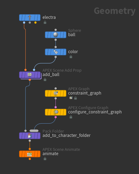
In this example, a ball is driven by two driver controls (Electra’s hands) in an animation scene. The ball also oscillates between the hand controls according to a sine function. Driver controls can be locators or character controls in an animation scene.
-
On the
Electra SOP, set Output to APEX Scene. -
Add the ball geometry to the scene using the
APEX Scene Add Prop SOP. In the Prop Name parameter, set the name of the ball that will appear in the selection sets. -
The
APEX Graph SOP brings in two matrices, start and end, as the drivers. The driven control’s position between the two drivers is determined using a sine function:
Constraint graph with driver controls -
The
StartandEndnodes are the two drivers. They come from the matrices in the graph input ports which we renamed to start and end. -
transform::Blend blends between the
StartandEndtransforms using thesine function as the blend value. The value of the sine function is modified to go from 0 to 1 instead of -1 to 1 because it is the input to transform::Blend’s blend port. -
Rename the graph output port to xform.
-
-
On the
APEX Configure Graph SOP:-
Set Mode to Constraints.
-
In the Name parameter, specify a name for the constraint. In our example, we set Name to
SineCharControl. -
Add a parameter for the radians input port. See the previous example.
-
-
Configure the driver controls using the APEX Configure Graph SOP - for the
Startdriver:-
In the Constraint Configuration section, click
beside Drivers. -
Set the Driver Name to
Start. -
Specify where the input data for the driver comes from - click
beside Input Bindings. -
Set To Port to
start. -
Set From Control to Driver: Start.
-
We want the start input port to have the driver’s transform data, so set Driver Data to Control Output and specify
xformin the textbox.Note
The
xformin this parameter is the world space transform of the driver - it is the xform output port of theTransformObject node that represents the driver (this TransformObject node is not shown in the constraint graph). This xformis not related to the xform port on the constraint graph’s output node.
Repeat the above steps for the
Enddriver. -
-
Add the constraint graph to the animation scene - on the
Pack Folder SOP:-
Set Parent Folder to
/constraints/library. -
Specify a name for the constraint graph. In our example, we set Name to
sinecharcontroland Type tograph.
-
-
On the
APEX Scene Animate SOP, enter the animate state and bring up the animate state parameters:-
In the Constraint tab, Parameters section, set Constraint to SineCharControl.
-
Below the Constraint menu, the controls are listed in the order they must be selected. Select the ball control, hold ⇧ Shift, select the start control, then select the end control. Press H over the viewport.
-
Select the constraint (in the selection sets or by clicking the dotted line).
-
In the animate state parameters, adjust the Radians parameter to move the ball between the hands.
In the video below, Electra’s hands drive the ball, and the ball moves between the hands as the Radians parameter is adjusted:
Ball driven by hand controls -
Adding controls to a constraint graph 
In this example, a ball is driven by two controls that are added to the constraint graph. We refer to these added controls as constraint controls. The ball also oscillates between the two controls according to a sine function. This uses the same network as a previous example.
-
In the
APEX Graph SOP, we add two controls, StartandEnd. The ball’s position between the two controls is determined using a sine function:
Add constraint controls -
Turn the
TransformObject nodes into controls by promoting their translate value (t input port). You can optionally rename the promoted ports on the graph input node. In our example, we name them start and end. The transform::Build nodes piped into the restlocal input on the TransformObject nodes set the initial position of the controls. -
The constraint’s inputs come from the input parameter (radians port) and controls (start and end ports) on the graph input node.
-
transform::Blend blends between the
StartandEndtransforms using thesine function as the blend value. The value of the sine function is modified to go from 0 to 1 instead of -1 to 1 because it is the input to transform::Blend’s blend port. -
Rename the graph output port to xform.
-
-
On the
APEX Configure Graph SOP:-
Set Mode to Constraints.
-
In the Name parameter, specify a name for the constraint. In our example, we set Name to
SineControl. -
Add a parameter for the radians input port. See the previous example.
There is no need to specify any input bindings because the constraint doesn’t need the transform data from any driven or driver controls.
Note
Controls created within a constraint graph (as TransformObject nodes) cannot be defined as “drivers” in a constraint, so in this example, we don’t need to add any Drivers.
-
-
Add the constraint graph to the animation scene - on the
Pack Folder SOP:-
Set Parent Folder to
/constraints/library. -
Specify a name for the constraint graph. In our example, we set Name to
sinecontrol, and Type tograph.
-
-
On the
APEX Scene Animate SOP, enter the animate state and bring up the animate state parameters:-
In the Constraint tab, Parameters section, set Constraint to SineControl.
-
The Radians parameter appears as a value you can control.
-
Select the ball control and press H over the viewport.
-
Adjust the Radians parameter to move the ball between the controls.
In the video below, the two white dots are the
StartandEndcontrols that drive the ball. The ball moves between the controls as the Radians parameter is adjusted:Ball driven by constraint controls -