| On this page | |
| Since | 18.0 |
The Gas Project Non Divergent Adaptive DOP removes divergence from a fluid’s velocity field. Divergence in a velocity represents expansion or contraction of the fluid volume. This divergence is projected out of the velocity field by computing a pressure field throughout the simulated fluid and then applying the gradient of the pressure field to the velocity field. The pressure field is solved on an adaptive (octree) background grid to significantly improve performance over solving with a uniform grid (as done in the ![]() Gas Project Non Divergent Variational DOP).
Gas Project Non Divergent Variational DOP).
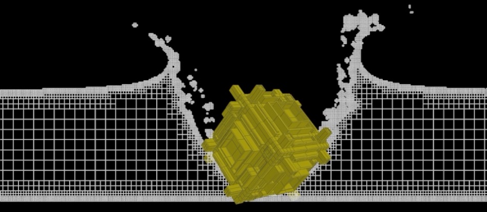
In order to maintain high resolution details in the simulation, a band of fine grid cells are constructed along the boundaries of the fluid. The grid is then progressively coarsened into the interior of the fluid. To minimize the difference between the adaptive and uniform grid pressure solves, the adaptive pressure is up-sampled and smoothed back to the uniform grid before updating the velocity field.
Note
You must turn on the Solve Pressure with Adaptivity checkbox on the FLIP Solver for adaptive pressure solving to work.
Parameters 
Velocity Field
The fluid velocity field to make divergence free (such as enforce incompressibility). This must be a vector field.
Surface Field
A signed distance field that specifies which voxels are inside the fluid (values less than or equal to zero) or outside the fluid (values greater than zero). Incompressibility is only enforced on the interior voxels.
Surface Weights Field
This field stores the percentage of fluid between pressure samples. It is usually computed with a ![]() Gas SDF To Fog DOP. This field should match the size and sampling of the velocity field.
Gas SDF To Fog DOP. This field should match the size and sampling of the velocity field.
Surface Pressure Field
This field is used to apply non-zero pressure at the fluid boundary. Surface pressure can be used to simulate phenomena like surface tension. This field should match the size and sampling of the surface field.
Collision Field
A signed distance field that specifies which voxels are inside the collision object (values greater than zero) or outside the collision object (values less than or equal to zero).
Collision Weights Field
This field stores the percentage that a face of a voxel is inside a collision object and is used to integrate the velocities for both the fluid and the collision when computing divergence per voxel. It is usually computed with a ![]() Gas SDF To Fog DOP.
Gas SDF To Fog DOP.
Collision Velocity Field
The velocities of the collision objects. If not provided, the collision velocities will be assumed to be zero.
Use Sharp Collisions
Sharp collision handling uses a cut-cell method to handle collisions more accurately. However, this can produce instabilities in the fluid velocity, so it is recommended to disable this feature unless better accuracy is required.
Goal Divergence Field
The intended purpose of this solver is to remove divergence from the velocity field. However, adding non-zero divergence into the simulation is possible with the goal divergence field. The field is scaled by the volume of the simulation voxels to function independent of the simulation resolution.
Custom Fine-cell Field
By default, the adaptive solver will construct fine-cells along the fluid boundary that match the simulation resolution and build coarse cells in the fluid interior. By specifying a custom field, fine cells will also be generated in the fluid interior for voxels in the custom field with values 1.
Pressure Field
The internal fluid pressure required to make the velocity field divergence free.
Use Pressure To Warm Start Solver
Uses pressure from the previous timestep as an initial guess for the solver. This will often provide faster solver convergence, resulting in faster simulation times.
Pressure in tanks of water increase from the top to the bottom. Frame to frame, this pressure gradient likely looks the same everywhere, so rather than starting from scratch, this option will try to re-use the previous pressure as a start condition. This causes it to find the final pressures faster, speeding up solve times. This is most effective in mostly static sims, especially deep tanks.
Density Field
The density (mass / volume) of the fluid. Not to be confused with the density field in smoke simulations. Only fluids with uniform density are currently supported. The values here will be clamped within the range specified by Min Density and Max Density.
Min Density
The values specified in the Density field will be lower-clamped to this value, specified in kilograms / meters^3.
Max Density
The values specified in the Density field will be upper-clamped to this value, specified in kilograms / meters^3.
Valid Field
A vector field that represents velocity samples that are updated to remove divergence. This field should match the size and sampling of the velocity field, with stored values of 0 representing invalid faces and 1 representing valid faces.
Surface Extrapolation Cells
To account for fluid pressure in voxels partially occupied by both fluid and collision surfaces, the fluid surface is extrapolated into the collision surface when constructing the pressure equations.
Error Tolerance
Tolerance specifies how much error is allowed when solving for pressure. Error results in divergence left over in the velocity field, which often causes volume changes over time. Smaller errors will take longer to converge but produce more accurate results.
Max Solver Iterations
The solver will stop after the maximum iteration limit has been reached, even if the error is above the specified tolerance. This limit should be set significantly higher than needed and only used as a fail-safe if the solver fails to converge.
Clean-up Smoother Iterations
The adaptive solver uses coarse cells inside the fluid when solving for pressure. The resulting pressure is then progressively up-sampled to the fine-cell cell level. To remove noise introduced from up-sampling, a number of smoother iterations are applied to the pressure after each up-sampling operation.
Use Gauss Seidel Smoother
During the up-sampling stage, pressure is smoothed using a parallel Jacobi smoother by default. This option enables a Gauss-Seidel smoother instead, which results in better noise reduction per smoother iteration. Both smoothers are implemented to maximize parallelism, so the cost per smoother iteration is similar.
Octree Levels
When solving for pressure, the interior of the fluid volume is filled with coarse cells. The largest allowable coarse cell in set by this level, where the width of the coarsest cell is larger than the simulation’s voxel size by a factor of 2xOctree Levels.
Fine-cell Bandwidth
In order to capture highly detailed fluid behavior, cells within a thin layer along the boundary of the fluid are kept at the finest resolution and interior cells are progressively coarsened until reaching the specified Octree Levels limit of coarsening.
Output Octree Visualization Geometry
For visualization and debugging purposes, enabling this option generates the underlying octree geometry. It does not produce the actual octree data structure, but rather a geometry of active cell center points to be used as a visual aid.
Only Generate Octree Geometry
For special circumstances where only the underlying octree geometry is required, the solver will terminate early, only generating the visualization geometry.
Octree Visualization Geometry
The geometry data to generate the octree visualization geometry with.
Use Waterline
See ![]() FLIP Solver.
FLIP Solver.
Waterline
See ![]() FLIP Solver.
FLIP Solver.
Waterline Direction
See ![]() FLIP Solver.
FLIP Solver.
Parameter Operations
Each data option parameter has an associated menu which specifies how that parameter operates.
Use Default
Use the value from the Default Operation menu.
Set Initial
Set the value of this parameter only when this data is created. On all subsequent timesteps, the value of this parameter is not altered. This is useful for setting up initial conditions like position and velocity.
Set Always
Always set the value of this parameter. This is useful when specific keyframed values are required over time. This could be used to keyframe the position of an object over time, or to cause the geometry from a SOP to be refetched at each timestep if the geometry is deforming.
You can also use this setting in
conjunction with the local variables for a parameter value to
modify a value over time. For example, in the X Position, an
expression like $tx + 0.1 would cause the object to
move 0.1 units to the right on each timestep.
Set Never
Do not ever set the value of this parameter. This option is most useful when using this node to modify an existing piece of data connected through the first input.
For example, an ![]() RBD State
DOP may want to animate just the mass of an
object, and nothing else. The Set Never option could be used
on all parameters except for Mass, which would use Set
Always.
RBD State
DOP may want to animate just the mass of an
object, and nothing else. The Set Never option could be used
on all parameters except for Mass, which would use Set
Always.
Default Operation
For any parameters with their Operation menu set to Use Default, this parameter controls what operation is used.
This parameter has the same menu options and meanings as the Parameter Operations menus, but without the Use Default choice.
Make Objects Mutual Affectors
All objects connected to the first input of this node become mutual affectors.
This is equivalent to using an ![]() Affector
DOP to create an affector relationship between
Affector
DOP to create an affector relationship between
* and * before connecting it to this node. This option makes it
convenient to have all objects feeding into a solver node affect
each other.
Group
When an object connector is attached to the first input of this node, this parameter can be used to choose a subset of those objects to be affected by this node.
Data Name
Indicates the name that should be used to attach the data to an object or other piece of data. If the Data Name contains a “/” (or several), that indicates traversing inside subdata.
For example, if the ![]() Fan Force DOP has the default Data Name
“Forces/Fan”. This attaches the data with the name “Fan” to an
existing piece of data named “Forces”. If no data named “Forces”
exists, a simple piece of container data is created to hold the
“Fan” subdata.
Fan Force DOP has the default Data Name
“Forces/Fan”. This attaches the data with the name “Fan” to an
existing piece of data named “Forces”. If no data named “Forces”
exists, a simple piece of container data is created to hold the
“Fan” subdata.
Different pieces of data have different requirements on what names should be used for them. Except in very rare situations, the default value should be used. Some exceptions are described with particular pieces of data or with solvers that make use of some particular type of data.
Unique Data Name
Turning on this parameter modifies the Data Name parameter value to ensure that the data created by this node is attached with a unique name so it will not overwrite any existing data.
With this parameter turned off, attaching two pieces of data with the same name will cause the second one to replace the first. There are situations where each type of behavior is desirable.
If an object
needs to have several ![]() Fan Forces blowing on it, it is
much easier to use the Unique Data Name feature to ensure that
each fan does not overwrite a previous fan rather than trying to
change the Data Name of each fan individually to avoid
conflicts.
Fan Forces blowing on it, it is
much easier to use the Unique Data Name feature to ensure that
each fan does not overwrite a previous fan rather than trying to
change the Data Name of each fan individually to avoid
conflicts.
On the other hand, if an object is known to have ![]() RBD
State data already attached to it, leaving this
option turned off will allow some new
RBD
State data already attached to it, leaving this
option turned off will allow some new ![]() RBD State
data to overwrite the existing data.
RBD State
data to overwrite the existing data.
Solver Per Object
The default behavior for solvers is to attach the exact same solver to all of the objects specified in the group. This allows the objects to be processed in a single pass by the solver, since the parameters are identical for each object.
However, some objects operate more logically on a single object at
a time. In these cases, one may want to use $OBJID expressions
to vary the solver parameters across the objects. Setting this
toggle will create a separate solver per object, allowing $OBJID
to vary as expected.
Setting this is also required if stamping the parameters with a Copy Data DOP.
Inputs 
All Inputs
Any microsolvers wired into these inputs will be executed prior to this node executing. The chain of nodes will thus be processed in a top-down manner.
Outputs 
First Output
The operation of this output depends on what inputs are connected to this node. If an object stream is input to this node, the output is also an object stream containing the same objects as the input (but with the data from this node attached).
If no object stream is
connected to this node, the output is a data output. This data
output can be connected to an ![]() Apply Data DOP,
or connected directly to a data input of another data node, to
attach the data from this node to an object or another piece of
data.
Apply Data DOP,
or connected directly to a data input of another data node, to
attach the data from this node to an object or another piece of
data.
Locals 
channelname
This DOP node defines a local variable for each channel and parameter on the Data Options page, with the same name as the channel. So for example, the node may have channels for Position (positionx, positiony, positionz) and a parameter for an object name (objectname).
Then there will also be local variables with the names positionx, positiony, positionz, and objectname. These variables will evaluate to the previous value for that parameter.
This previous value is always stored as part of the data attached to the object being processed. This is essentially a shortcut for a dopfield expression like:
dopfield($DOPNET, $OBJID, dataName, "Options", 0, channelname)
If the data does not already exist, then a value of zero or an empty string will be returned.
DATACT
This value is the simulation time (see variable ST) at which the current data was created. This value may not be the same as the current simulation time if this node is modifying existing data, rather than creating new data.
DATACF
This value is the simulation frame (see variable SF) at which the current data was created. This value may not be the same as the current simulation frame if this node is modifying existing data, rather than creating new data.
RELNAME
This value will be set only when data is being attached to a relationship (such as when Constraint Anchor DOP is connected to the second, third, of fourth inputs of a Constraint DOP).
In this case, this value is set to the name of the relationship to which the data is being attached.
RELOBJIDS
This value will be set only when data is being attached to a relationship (such as when Constraint Anchor DOP is connected to the second, third, of fourth inputs of a Constraint DOP).
In this case, this value is set to a string that is a space separated list of the object identifiers for all the Affected Objects of the relationship to which the data is being attached.
RELOBJNAMES
This value will be set only when data is being attached to a relationship (such as when Constraint Anchor DOP is connected to the second, third, of fourth inputs of a Constraint DOP).
In this case, this value is set to a string that is a space separated list of the names of all the Affected Objects of the relationship to which the data is being attached.
RELAFFOBJIDS
This value will be set only when data is being attached to a relationship (such as when Constraint Anchor DOP is connected to the second, third, of fourth inputs of a Constraint DOP).
In this case, this value is set to a string that is a space separated list of the object identifiers for all the Affector Objects of the relationship to which the data is being attached.
RELAFFOBJNAMES
This value will be set only when data is being attached to a relationship (such as when Constraint Anchor DOP is connected to the second, third, of fourth inputs of a Constraint DOP).
In this case, this value is set to a string that is a space separated list of the names of all the Affector Objects of the relationship to which the data is being attached.
ST
The simulation time for which the node is being evaluated.
Depending on the settings of the ![]() DOP Network
Offset Time and Scale Time parameters,
this value may not be equal to the current Houdini time
represented by the variable T.
DOP Network
Offset Time and Scale Time parameters,
this value may not be equal to the current Houdini time
represented by the variable T.
ST is guaranteed to have a value of zero at the
start of a simulation, so when testing for the first timestep of a
simulation, it is best to use a test like $ST == 0, rather than
$T == 0 or $FF == 1.
SF
The simulation frame (or more accurately, the simulation time step number) for which the node is being evaluated.
Depending on the settings of the ![]() DOP Network parameters,
this value may not be equal to the current Houdini frame number
represented by the variable F. Instead, it is equal to
the simulation time (ST) divided by the simulation timestep size
(TIMESTEP).
DOP Network parameters,
this value may not be equal to the current Houdini frame number
represented by the variable F. Instead, it is equal to
the simulation time (ST) divided by the simulation timestep size
(TIMESTEP).
TIMESTEP
The size of a simulation timestep. This value is useful for scaling values that are expressed in units per second, but are applied on each timestep.
SFPS
The inverse of the TIMESTEP value. It is the number of timesteps per second of simulation time.
SNOBJ
The number of objects in the simulation. For nodes that
create objects such as the ![]() Empty Object DOP,
SNOBJ increases for each object that is evaluated.
Empty Object DOP,
SNOBJ increases for each object that is evaluated.
A good way to guarantee unique object names is to use an expression
like object_$SNOBJ.
NOBJ
The number of objects that are evaluated by the current node during this timestep. This value is often different from SNOBJ, as many nodes do not process all the objects in a simulation.
NOBJ may return 0 if the node does not
process each object sequentially (such as the ![]() Group
DOP).
Group
DOP).
OBJ
The index of the specific object being processed by the node. This value always runs from zero to NOBJ-1 in a given timestep. It does not identify the current object within the simulation like OBJID or OBJNAME; it only identifies the object’s position in the current order of processing.
This value is useful for generating a
random number for each object, or simply splitting the objects into
two or more groups to be processed in different ways. This value
is -1 if the node does not process objects sequentially (such
as the ![]() Group DOP).
Group DOP).
OBJID
The unique identifier for the object being processed. Every object is assigned an integer value that is unique among all objects in the simulation for all time. Even if an object is deleted, its identifier is never reused. This is very useful in situations where each object needs to be treated differently, for example, to produce a unique random number for each object.
This value is also the best way to look up information on an object using the dopfield expression function.
OBJID is -1 if the node does not process objects
sequentially (such as the ![]() Group DOP).
Group DOP).
ALLOBJIDS
This string contains a space-separated list of the unique object identifiers for every object being processed by the current node.
ALLOBJNAMES
This string contains a space-separated list of the names of every object being processed by the current node.
OBJCT
The simulation time (see variable ST) at which the current object was created.
To check if an object was created
on the current timestep, the expression $ST == $OBJCT should
always be used.
This value is zero if the node does not process
objects sequentially (such as the ![]() Group DOP).
Group DOP).
OBJCF
The simulation frame (see variable SF) at which the current object was created. It is equivalent to using the dopsttoframe expression on the OBJCT variable.
This value is zero if the node does not process objects
sequentially (such as the ![]() Group DOP).
Group DOP).
OBJNAME
A string value containing the name of the object being processed.
Object names are not guaranteed to be unique within a simulation. However, if you name your objects carefully so that they are unique, the object name can be a much easier way to identify an object than the unique object identifier, OBJID.
The object name can
also be used to treat a number of similar objects (with the same
name) as a virtual group. If there are 20 objects named “myobject”,
specifying strcmp($OBJNAME, "myobject") == 0 in the activation field
of a DOP will cause that DOP to operate on only those 20 objects.
This value is the empty string if the node does not process objects
sequentially (such as the ![]() Group DOP).
Group DOP).
DOPNET
A string value containing the full path of the current DOP network. This value is most useful in DOP subnet digital assets where you want to know the path to the DOP network that contains the node.
Note
Most dynamics nodes have local variables with the same names as the
node’s parameters. For example, in a ![]() Position DOP,
you could write the expression:
Position DOP,
you could write the expression:
$tx + 0.1
…to make the object move 0.1 units along the X axis at each timestep.