| On this page | |
| Since | 14.0 |
POP Source is a node that generates particles from geometry, often a referenced SOP network.
Using Source 
-
Create an object.
-
Click the
 Source tool on the Particles tab.
 The
 particle system will attach itself to the object you have selected.
 -
Click
 play to see the particles.
Parameters 
Source 
Emission Type
Where on the source geometry to emit points from.
All Points
All of the points will emit points simultaneously.
All Geometry
All of the source object will be added to the particle system. This includes non-points, such as primitives. This is useful for bringing in constraints or other geometry information. Note that most POPs just work on points, ignoring any attached geometry.
Points
The desired number of points will be emitted from random source points.
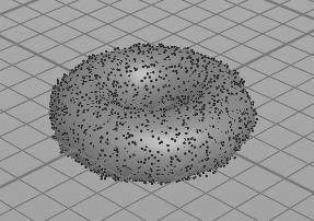
Scatter onto Surfaces
The desired number of points will be emitted from random locations on the surfaces of the geometry.
Geometry Source
Specifies the SOP to use.
Use Parameter Values
Use the SOP specified in the SOP parameter below.
Use DOP Object
Use the named DOP object in this DOP network.
Use First Context Geometry
Use the SOP connected to the DOP network’s first input.
Use Second Context Geometry
Use the SOP connected to the DOP network’s second input.
Use Third Context Geometry
Use the SOP connected to the DOP network’s third input.
Use Fourth Context Geometry
Use the SOP connected to the DOP network’s fourth input.
SOP
Path to the SOP (when Geometry Source is set to Use Parameter Values).
DOP Objects
Name of DOP Objects (When Geometry Source is set to Use DOP Object).
Use Object Transform
When Geometry Source is set to Use Parameter Values, the transform of the object containing the chosen SOP is applied to the geometry. This is useful if the location of the geometry is defined by an object transform.
Emission Attribute
When in surface mode, this point attribute will be used to vary the chance of any polygon from emitting points. Higher values will increase the relative chance of that polygon getting an emission.
Relax Iterations
New points will be spread out from each other. This is done in successive passes, so the more iterations, the more equally spaced the sourced particles will be. This may result in points matching frame to frame if they get over constrained, however.
Scale Radii By
Point radii will be scaled by this before any relaxing of the points. Specifying a scale less than 1 will increase “clumpiness” of the resulting points, with a value of zero resulting in no relaxation. Specifying a scale greater than 1 may speed up convergence of the relaxation, especially when scattering on curves.
After any scaling, Max Relax Radius will be enforced before any relaxation.
Max Relax Radius
This must be set appropriately to prevent outlier points in low-density areas causing problems when relaxing points.
In order to approximately maintain variations in density, points are assigned radii inversely proportional to density (for curves), the square root of density (for surfaces), or the cube root of density (for volumes). This may cause problems for areas whose densities are near zero, especially in volumes, when painting density on a surface, or when using a density texture with a black background, since the radius approaches infinity. This parameter specifies the maximum radius within which points will influence other points.
When this is disabled, there will still be a maximum radius, which is currently chosen as half the diagonal length of the bounding box of the input geometry.
Scale Point Count by Area
When in surface mode, the constant and impulse point counts will be scaled by the total area (taking into account any emission attribute) of the geometry. This lets you paint an emission density and have the number of particles increase as the area of emission increases.
Reference Area
The impulse and constant emission values are often set for an entire object, which is often larger than a unit area. Therefore, this acts as a scale on their values before applying the area count.
An object of the size of Reference Area will emit at the specified impulse/constant rate. A larger object will emit proportionally more particles, and a smaller one less.
Remove Overlapping
Potential new particles are compared against the existing set of particles.
If their pscale attribute overlaps, the new particle isn’t added.
This can be useful to continuously add new particles to a sand simulation without creating explosions from overlaps.
Note this only tests against particles that already exist, so it is important the set of new sourced particles don’t overlap within themselves.
Birth 
This operator has two methods for emitting particles. You can use these methods together or separately:
-
Impulse creates a certain number of particles each time the node cooks.
-
Constant creates a certain number of particles per second.
Impulse Activation
Turns impulse emission on and off. Impulse emits the number of particles in the Impulse Birth Rate below each time the operator cooks. A value of 0 means off, any other value means on.
Impulse Count
Number of particles to emit each time the node cooks (when Impulse activation is on).
Const. Activation
Turns constant emission on and off. Impulse emits the number of particles in the Constant birth rate below each second. A value of 0 means off, any other value means on.
Const. Birth Rate
Number of particles to emit per second (when Constant Activation is on).
Max Sim Points
This parameter is a cap on the total number of points in the bound geometry. If this limiting is enabled, then the emitter will not create any more particles once the specified maximum is reached.
Max Points per Frame
Limit on the number of points that can be added each frame. This option can be used to prevent the emitter from spawning an undesirably large amount of particles as a result of errant parameter values.
Probabilistic Emission
Emit particles by treating the birth rate as a probability. If enabled, particle emission will be distributed randomly across timesteps when the birth rate is low. If disabled, the emission will occur at regular intervals. For example, with a Constant Birth Rate of 1 and Probabilistic Emission enabled, you will see particles emitted at random intervals but an overall rate of approximately 1 per second. With Probabilistic Emission disabled, particles will be emitted at each one-second interval.
Just Born Group
Name of a group to put the new points into. The particles will only be in this group the same substep that they were created.
Life Expectancy
How long the particle will live (in seconds).
Life Variance
Particles will live the number of seconds in Life Expectancy, plus or minus this number of seconds. Use 0 for no variance.
Jitter Birth Time
Rather than have the particles all be created with an age of 0, they are created with a random age within the current timestep. They will also be moved by their starting velocity times this age. This is useful when adding high velocity particles from emitters as it won’t generate clumps on each frame.
Interpolate Source
The source can also be interpolated linearly to better birth particles from fast moving sources. This uses the Jitter Birth Time to decide where in the source to interpolate. If you are wiring your source into the post solve, the Positive birth time and Backwards source should be used, which is useful since it does not require future knowledge of the source. However, to avoid clumping when large forces are present, you should use Negative birth time and Forward source. This requires you to delete all particles with negative age when rendering. Alternatively, you can wire into the Pre-Solve, and then use the Forward source with Negative birth time and not have to worry about seeing particles with negative age. However, this requires a source that you can compute outside the simulation.
Interpolation Method
The Interpolate Source takes two geometries and has to find a way to determine the in-between values of those geometries. If point counts and polygons match, the Match Topology option can be used for the most accurate result. Otherwise, point velocities may be computed with the Trail SOP and then Use Point Velocities selected. In this latter case, only one of the input geometries is needed, but the Forward and Backwards options are still used to determine if the born points lead or trail the object.
Attributes 
The parameters on this tab let you control which and how attributes are initialized on the emitted particles.
Initial State
If the emission type is Scatter on Surfaces, and the source is a SOP Path, the initial state of the particles can be set to sliding, stuck, or stopped.
Particles can then be released by setting the i@sliding, i@stuck, or i@stopped attributes to 0.
Inherit Attributes
This specifies which attributes to inherit from the source geometry.
Velocity
Set or add to velocity attribute.
Variance
Variance to velocity set above. The node will add +/- from 0 to this number along each axis to the Velocity parameter.
Ellipsoid Distribution
By default, the variance (if any) is distributed in a box, the size of which is determined by the Variance parameter. When this option is on, the variance is distributed in an ellipsoid instead.
Add ID Attributes
Add ID and parent attributes to the created particles.
Stream 
Stream Name
The name of the stream to be generated by this generator.
This value is prefixed with stream_ to form a group name
that all particles that belong to this logical stream will
be made part of.
Inputs 
Outputs 
First Output
The output of this node should be wired into a solver chain.
Merge nodes can be used to combine multiple solver chains.
The final wiring should go into one of the purple inputs of a full-solver, such as ![]() POP Solver or
POP Solver or ![]() FLIP Solver.
FLIP Solver.
Locals 
channelname
This DOP node defines a local variable for each channel and parameter on the Data Options page, with the same name as the channel. So for example, the node may have channels for Position (positionx, positiony, positionz) and a parameter for an object name (objectname).
Then there will also be local variables with the names positionx, positiony, positionz, and objectname. These variables will evaluate to the previous value for that parameter.
This previous value is always stored as part of the data attached to the object being processed. This is essentially a shortcut for a dopfield expression like:
dopfield($DOPNET, $OBJID, dataName, "Options", 0, channelname)
If the data does not already exist, then a value of zero or an empty string will be returned.
DATACT
This value is the simulation time (see variable ST) at which the current data was created. This value may not be the same as the current simulation time if this node is modifying existing data, rather than creating new data.
DATACF
This value is the simulation frame (see variable SF) at which the current data was created. This value may not be the same as the current simulation frame if this node is modifying existing data, rather than creating new data.
RELNAME
This value will be set only when data is being attached to a relationship (such as when Constraint Anchor DOP is connected to the second, third, of fourth inputs of a Constraint DOP).
In this case, this value is set to the name of the relationship to which the data is being attached.
RELOBJIDS
This value will be set only when data is being attached to a relationship (such as when Constraint Anchor DOP is connected to the second, third, of fourth inputs of a Constraint DOP).
In this case, this value is set to a string that is a space separated list of the object identifiers for all the Affected Objects of the relationship to which the data is being attached.
RELOBJNAMES
This value will be set only when data is being attached to a relationship (such as when Constraint Anchor DOP is connected to the second, third, of fourth inputs of a Constraint DOP).
In this case, this value is set to a string that is a space separated list of the names of all the Affected Objects of the relationship to which the data is being attached.
RELAFFOBJIDS
This value will be set only when data is being attached to a relationship (such as when Constraint Anchor DOP is connected to the second, third, of fourth inputs of a Constraint DOP).
In this case, this value is set to a string that is a space separated list of the object identifiers for all the Affector Objects of the relationship to which the data is being attached.
RELAFFOBJNAMES
This value will be set only when data is being attached to a relationship (such as when Constraint Anchor DOP is connected to the second, third, of fourth inputs of a Constraint DOP).
In this case, this value is set to a string that is a space separated list of the names of all the Affector Objects of the relationship to which the data is being attached.
ST
The simulation time for which the node is being evaluated.
Depending on the settings of the ![]() DOP Network
Offset Time and Scale Time parameters,
this value may not be equal to the current Houdini time
represented by the variable T.
DOP Network
Offset Time and Scale Time parameters,
this value may not be equal to the current Houdini time
represented by the variable T.
ST is guaranteed to have a value of zero at the
start of a simulation, so when testing for the first timestep of a
simulation, it is best to use a test like $ST == 0, rather than
$T == 0 or $FF == 1.
SF
The simulation frame (or more accurately, the simulation time step number) for which the node is being evaluated.
Depending on the settings of the ![]() DOP Network parameters,
this value may not be equal to the current Houdini frame number
represented by the variable F. Instead, it is equal to
the simulation time (ST) divided by the simulation timestep size
(TIMESTEP).
DOP Network parameters,
this value may not be equal to the current Houdini frame number
represented by the variable F. Instead, it is equal to
the simulation time (ST) divided by the simulation timestep size
(TIMESTEP).
TIMESTEP
The size of a simulation timestep. This value is useful for scaling values that are expressed in units per second, but are applied on each timestep.
SFPS
The inverse of the TIMESTEP value. It is the number of timesteps per second of simulation time.
SNOBJ
The number of objects in the simulation. For nodes that
create objects such as the ![]() Empty Object DOP,
SNOBJ increases for each object that is evaluated.
Empty Object DOP,
SNOBJ increases for each object that is evaluated.
A good way to guarantee unique object names is to use an expression
like object_$SNOBJ.
NOBJ
The number of objects that are evaluated by the current node during this timestep. This value is often different from SNOBJ, as many nodes do not process all the objects in a simulation.
NOBJ may return 0 if the node does not
process each object sequentially (such as the ![]() Group
DOP).
Group
DOP).
OBJ
The index of the specific object being processed by the node. This value always runs from zero to NOBJ-1 in a given timestep. It does not identify the current object within the simulation like OBJID or OBJNAME; it only identifies the object’s position in the current order of processing.
This value is useful for generating a
random number for each object, or simply splitting the objects into
two or more groups to be processed in different ways. This value
is -1 if the node does not process objects sequentially (such
as the ![]() Group DOP).
Group DOP).
OBJID
The unique identifier for the object being processed. Every object is assigned an integer value that is unique among all objects in the simulation for all time. Even if an object is deleted, its identifier is never reused. This is very useful in situations where each object needs to be treated differently, for example, to produce a unique random number for each object.
This value is also the best way to look up information on an object using the dopfield expression function.
OBJID is -1 if the node does not process objects
sequentially (such as the ![]() Group DOP).
Group DOP).
ALLOBJIDS
This string contains a space-separated list of the unique object identifiers for every object being processed by the current node.
ALLOBJNAMES
This string contains a space-separated list of the names of every object being processed by the current node.
OBJCT
The simulation time (see variable ST) at which the current object was created.
To check if an object was created
on the current timestep, the expression $ST == $OBJCT should
always be used.
This value is zero if the node does not process
objects sequentially (such as the ![]() Group DOP).
Group DOP).
OBJCF
The simulation frame (see variable SF) at which the current object was created. It is equivalent to using the dopsttoframe expression on the OBJCT variable.
This value is zero if the node does not process objects
sequentially (such as the ![]() Group DOP).
Group DOP).
OBJNAME
A string value containing the name of the object being processed.
Object names are not guaranteed to be unique within a simulation. However, if you name your objects carefully so that they are unique, the object name can be a much easier way to identify an object than the unique object identifier, OBJID.
The object name can
also be used to treat a number of similar objects (with the same
name) as a virtual group. If there are 20 objects named “myobject”,
specifying strcmp($OBJNAME, "myobject") == 0 in the activation field
of a DOP will cause that DOP to operate on only those 20 objects.
This value is the empty string if the node does not process objects
sequentially (such as the ![]() Group DOP).
Group DOP).
DOPNET
A string value containing the full path of the current DOP network. This value is most useful in DOP subnet digital assets where you want to know the path to the DOP network that contains the node.
Note
Most dynamics nodes have local variables with the same names as the
node’s parameters. For example, in a ![]() Position DOP,
you could write the expression:
Position DOP,
you could write the expression:
$tx + 0.1
…to make the object move 0.1 units along the X axis at each timestep.